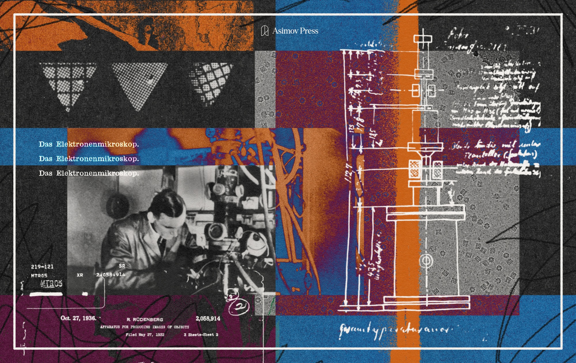
Making the Electron Microscope
Words by
Smrithi Sunil
Biological structures exist across a vast range of scales. At one end are whole organisms, varying in size from bacteria only a few micrometers across to mammals measured in feet.1 These can be seen with the naked eye or with simple light microscopes, which have been in use since the mid-1600s. At the smaller end, however, are atoms, amino acids, and proteins, spanning angstroms2 to nanometers in size.
Observing molecules at this smaller scale allows us to untangle the finer mechanisms of life: how individual neurons connect and communicate, how the ribosomal machinery translates genetic code into proteins, or how viruses like HIV invade and hijack host cells. Resolving fine structures, whether the double membrane of a chloroplast, the protein shell of a bacteriophage, or the branching architecture of a synapse, provides the bridge between atomic detail and whole-organism physiology, taking us from form to function.

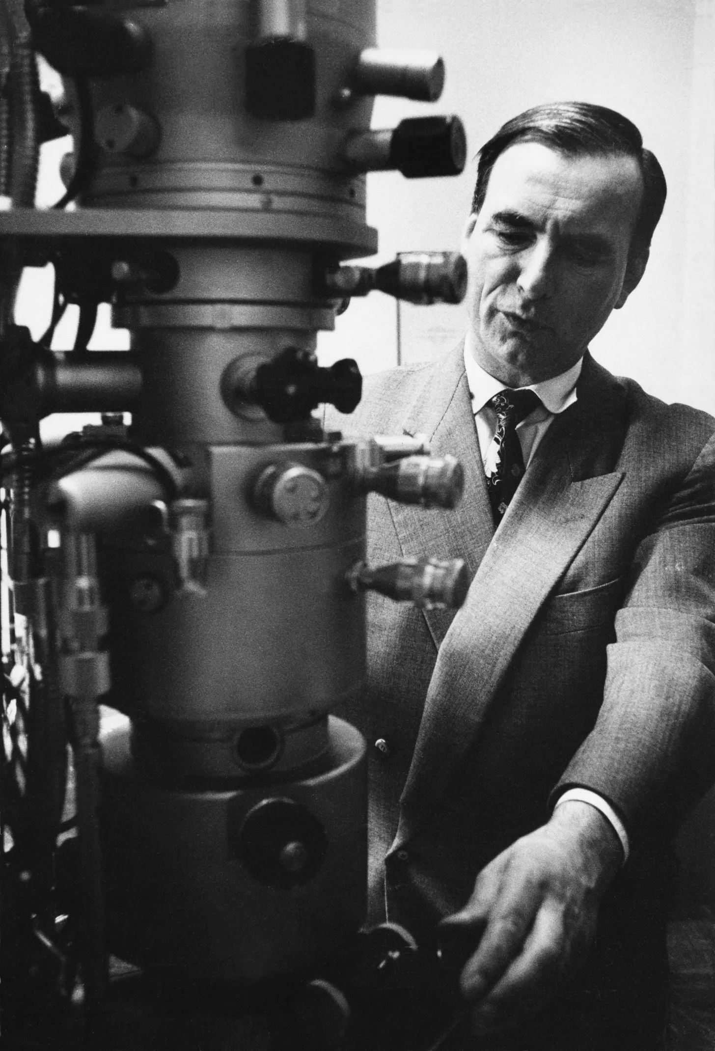
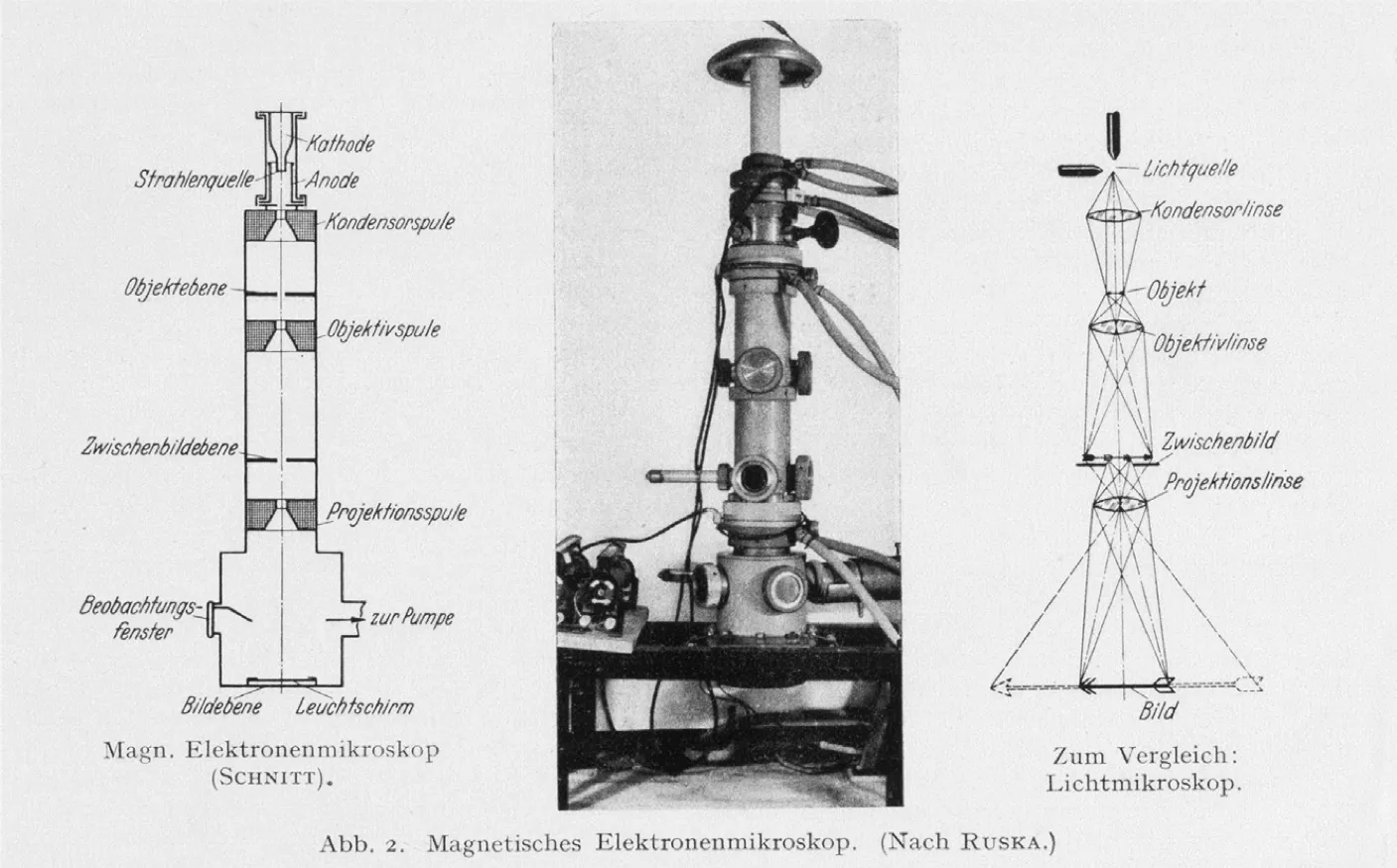
The ability to explore and map such minute mechanisms eluded scientists until the invention of the electron microscope. Conceived in the 1930s, it promised theoretical resolutions on the order of angstroms, nearly a hundred times finer than the most advanced light microscope of that era. In 1931, Ernst Ruska and his advisor Max Knoll, working at the Technical University in Berlin, designed the first prototype by replacing glass lenses with electromagnetic coils to focus beams of electrons instead of light.
That first instrument barely outperformed a magnifying glass in terms of resolution. But over the next century, refinements in design, sample preparation, and computation transformed the electron microscope into an indispensable tool for modern biology.
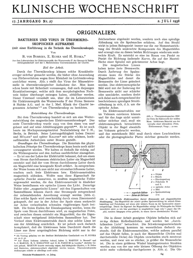
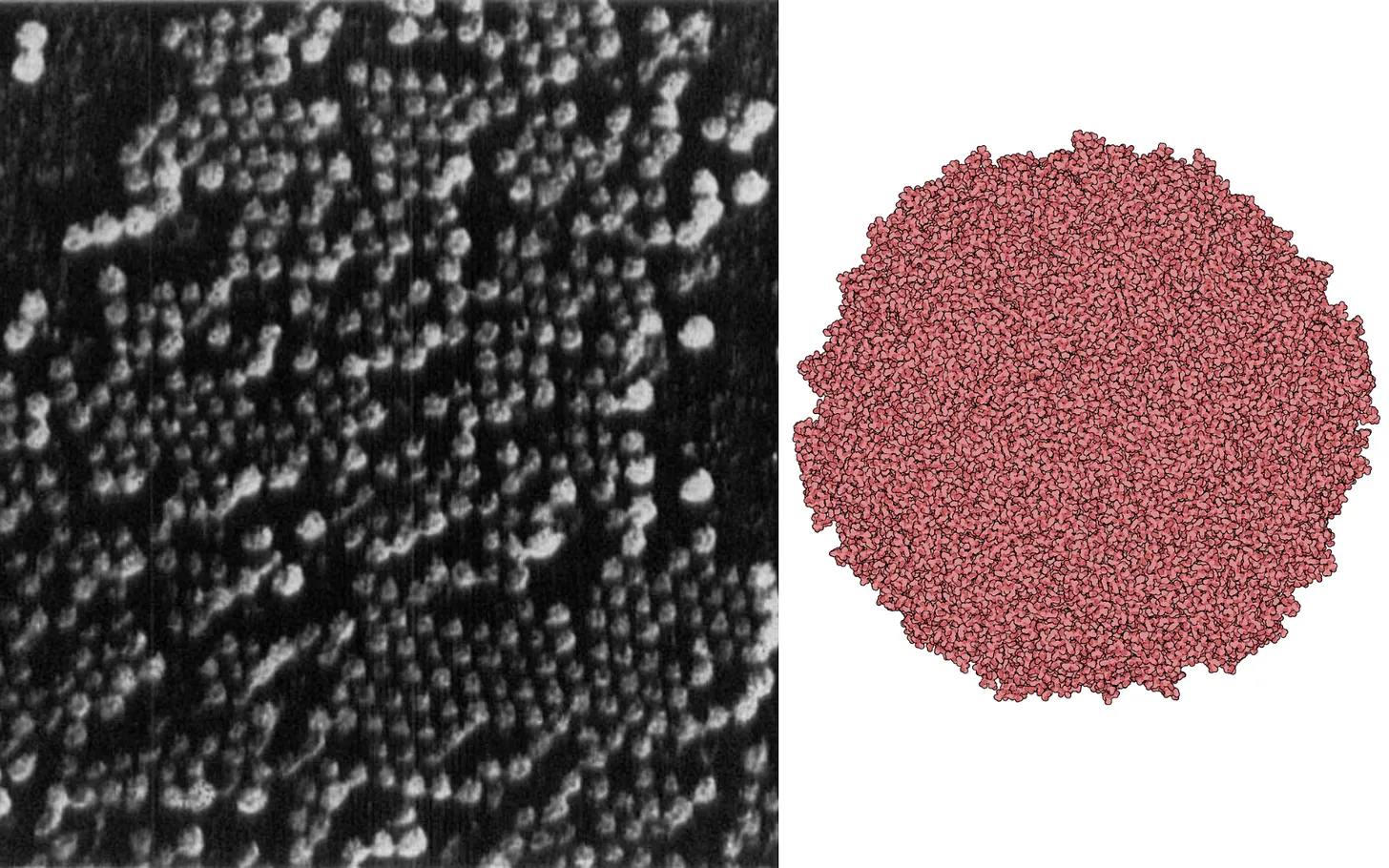
By 1938, scientists used an electron microscope to take a photograph of a virus — the mouse ectromelia orthopoxvirus — for the first time.3 And today, modern cryo-electron microscopy, in which samples are frozen in liquid ethane prior to imaging, can resolve individual atoms within proteins. During the COVID-19 pandemic, cryo-electron microscopy revealed the spike protein in the SARS-CoV-2 virus, which directly influenced the development of COVID vaccines. The technique also revealed a protein receptor that senses heat and pain, demonstrating how it translates physical signals to our nervous system, a breakthrough discovery that earned the 2021 Nobel Prize in Physiology.
Even as electron microscopes have allowed us to view ever smaller structures with clarity, challenges remain. One is that the images remain limited to static snapshots. Because samples must be imaged in a vacuum, it is impossible to directly observe the dynamism of live cells.4 In addition, specimens must be extremely thin to allow the electron beam to pass through, which prevents imaging of thick tissues. And finally, beyond these biological constraints, electron microscopes are physically large, can cost millions of dollars, and demand specialized facilities, training, and expertise to operate.
Despite these limitations, electron microscopy remains a powerful tool in biology, bridging the scales between molecular structure and living function. The story of its discovery is one of persistent ingenuity, involving a large cast of characters and numerous breakthroughs that helped make the modern electron microscope possible.
{{signup}}
By the late 19th century, biologists knew they were approaching the resolution limit of the light microscope. In their quest to see biology in finer detail, they had reached a barrier that light could not cross.
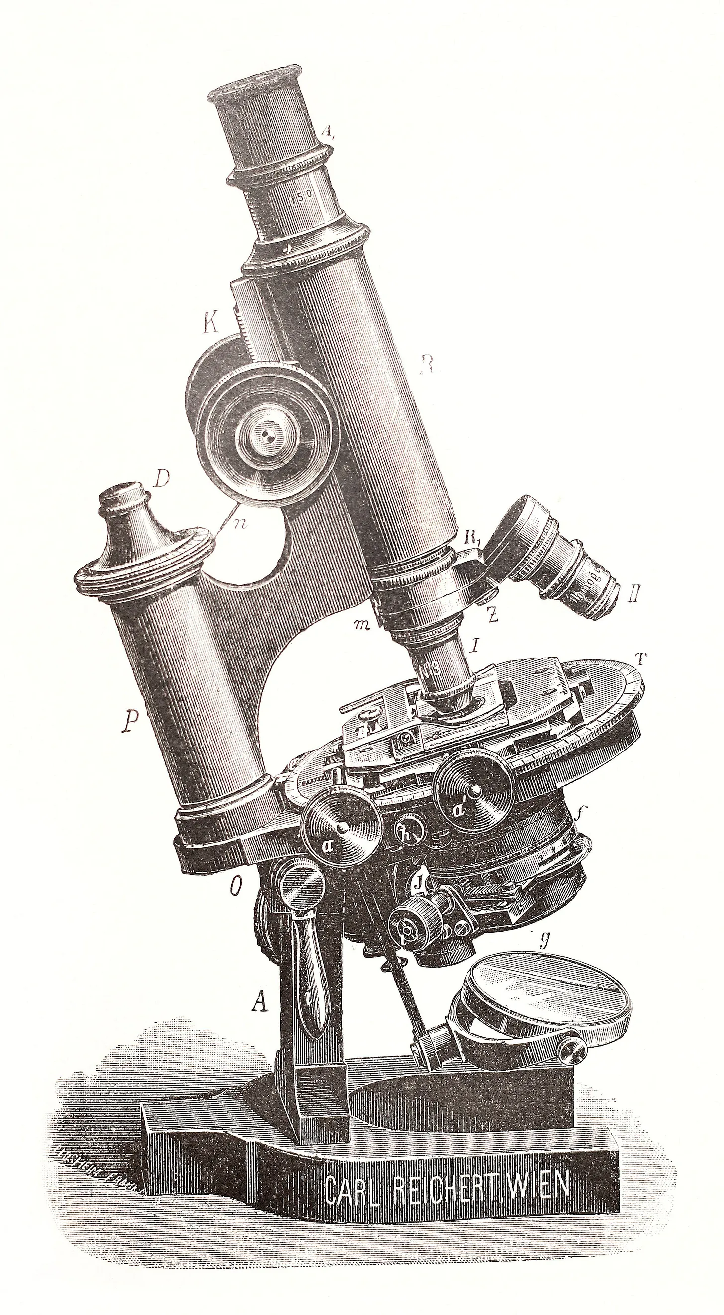
Proof of this came from Ernst Abbe, a professor of experimental physics and mathematics at the University of Jena in Germany. Until Abbe, microscope design had been more of an art than a science, with innovators building optical instruments through trial and error. Carl Zeiss, who had begun manufacturing microscopes in the 1850s, approached Abbe in 1866 about using his scientific expertise for the construction of microscopes. Together, they began developing tools to improve the uniformity and quality of optical lenses.
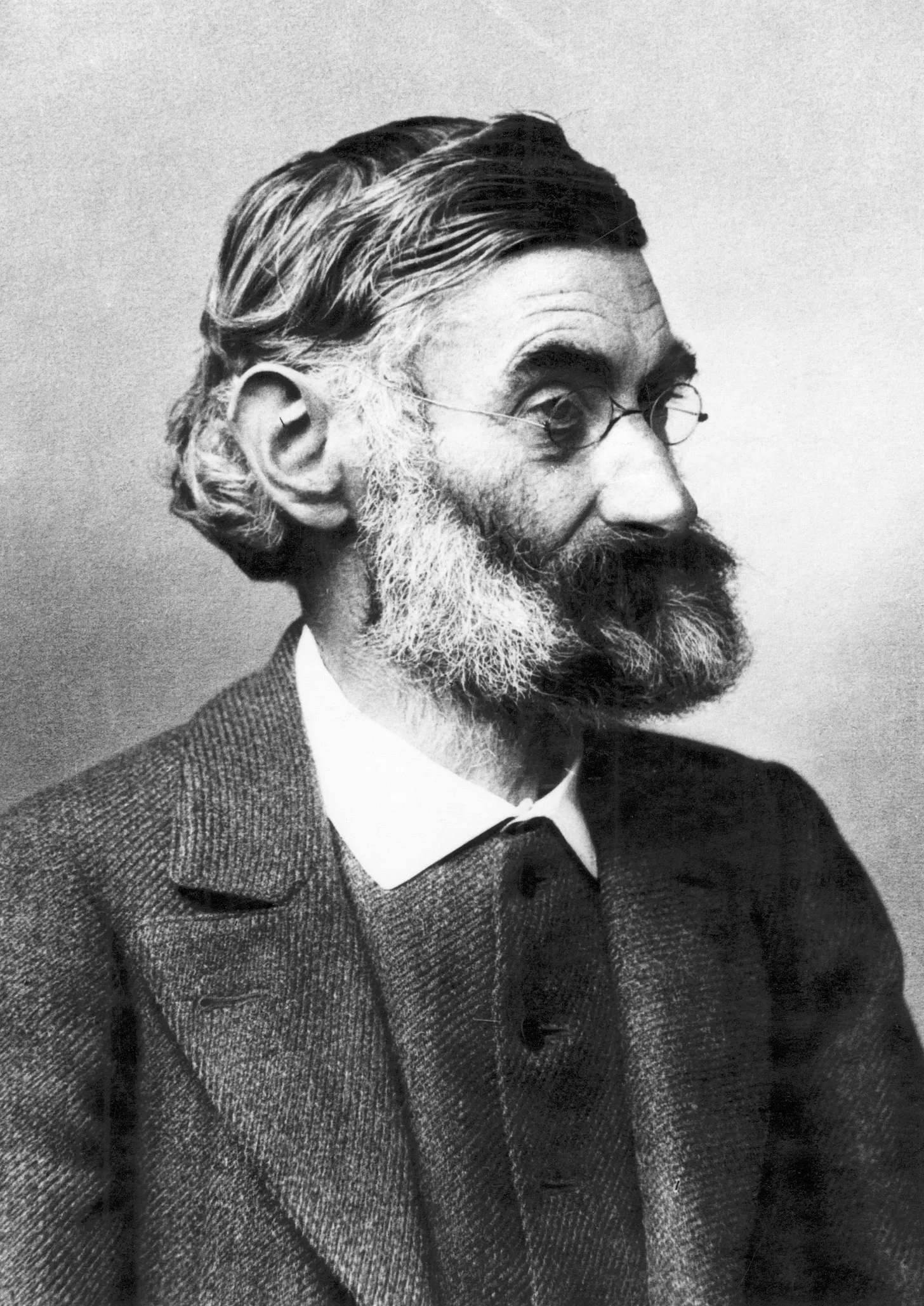
In the early 1870s, while working on the microscope objectives (the lens closest to the specimen in a microscope), Abbe discovered that the sharpness of an image did not only depend on how perfectly a lens was ground but also on how much diffracted light from the specimen the lens could capture. He realized that fine details in a specimen bend light into wide angles, and only objectives with a sufficiently large opening could collect those rays to bring the image into focus.
From this insight, Abbe defined the concept of the “numerical aperture” (a measure of how much light a lens can gather5) and showed that the smallest visible detail is limited by the wavelength of light divided by twice this value.6 Even with ultraviolet light, at the short end of the visible spectrum (400 nanometers), the limit of resolution was 200 nanometers — larger than most viruses, intracellular structures, and protein complexes.
Hope of resolving structures beneath this resolution boundary only arrived in 1895, when the German physicist Wilhelm Röntgen discovered X-rays, a form of high-energy electromagnetic radiation with wavelengths shorter than those of ultraviolet light, and published a (now-iconic) image of his wife Bertha’s hand, with her bones and wedding ring clearly visible. This was the first time the hidden insides of the body could be seen without dissection. The bones, joints, and even metal fragments lodged inside the body could be made visible.
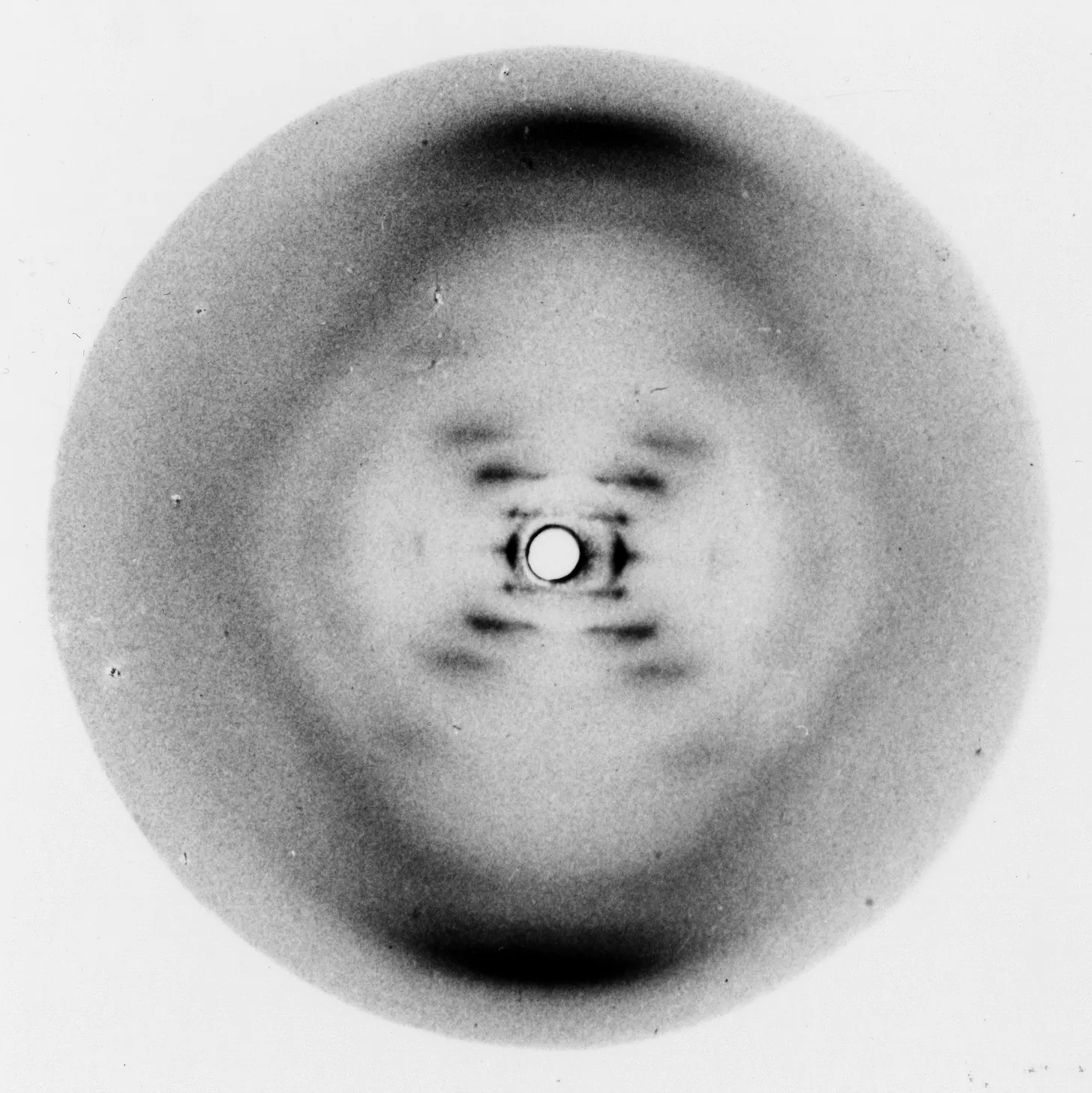
Between 1913 and 1915, the British physicist William Henry Bragg and his son, William Lawrence Bragg, developed a technique called X-ray crystallography. Working with simple crystals such as salt and diamond, they showed that when X-rays strike a regularly ordered crystal lattice, they diffract at specific angles that reveal the spacing of atoms within the crystal. The method works because X-rays have wavelengths about the size of chemical bonds, allowing the beams to reach and bounce off each atom in the lattice, reflecting the structure at an atomic scale. By applying a mathematical operation called a Fourier transform to these diffraction patterns captured on photographic plates, the Braggs reconstructed the three-dimensional arrangements of the atoms in the crystal.
Biomolecules, however, are not naturally crystalline. To study them, they had to be laboriously extracted, purified, and crystallized, separating them from their environment. The X-ray crystallography of biomolecules began in the 1930s, ushering in the field of structural biology. With sub-nanometer resolution, the invention of X-ray crystallography enabled a revolution in molecular biology. It was applied, for example, to solve the structures of DNA, hemoglobin, and insulin, molecules that have shaped the trajectory of modern biology.
But many biological targets remained out of reach. Viruses could rarely be crystallized, and cellular structures often lost their integrity when removed from their natural contexts. Thus, even with X-ray crystallography revealing the structures of small proteins and light microscopy capable of imaging cells, a gulf persisted between the study of small molecules and whole cells, which left much of biology invisible.
Meanwhile, access to the parallel world of electrons was beginning to open. At the turn of the 20th century, Hans Busch, a German physicist at the University of Jena, was studying how electron beams behaved in magnetic fields. His work built on decades of experiments with cathode rays, streams of electrons released when a high voltage is applied inside a glass tube.
Cathode rays had become central to both physics and technology: Physicists used them to probe how electrons scattered, ionized gases, and responded to electric and magnetic fields, and engineers used them to form the basis of devices such as the radio and television. It was while trying to better understand and control these beams that Busch postulated his remarkable theories.
In 1926 and 1927, Busch published two papers demonstrating mathematically that a magnetic coil could focus an electron beam in the same manner that a glass lens focuses light. While it was already known that coils could bend electron beams,7 Busch’s key insight was to frame this behavior in the language of optics: Electron beams could be treated like light rays. Concepts such as focal length, magnification, image formation, and even lens aberrations could all be applied to electrons. This meant that the well-developed theory of optical systems could be imported almost directly to other disciplines.
The Nobel Prize–winning physicist and inventor of holography, Denis Gabor, later reflected on Busch’s contribution in a 1942 lecture: “Busch’s paper was more than an eye-opener; it was almost like a spark in an explosive mixture. In 1927, the situation in physics was such that nothing more than the words ‘electron lens’ were needed to start a real burst of creative activity.”
And so it was that Busch’s idea sparked the birth of electron optics. Within a few years, at least three independent inventors would lay claim to having designed the electron microscope, all tracing their inspiration back to his initial insight.
{{signup}}
In 1928, the High Tension Laboratory at the Technical University in Berlin (a premier research facility focused on electrical engineering in the interwar years) was researching high-voltage power transmission and insulation. A persistent obstacle was the electrical surge often caused by thunderstorms, which repeatedly damaged the lab’s equipment. But before scientists could design a way to mitigate the problem, they first needed to understand it: Exactly when did these surges occur, and how fast or large were the voltage fluctuations?
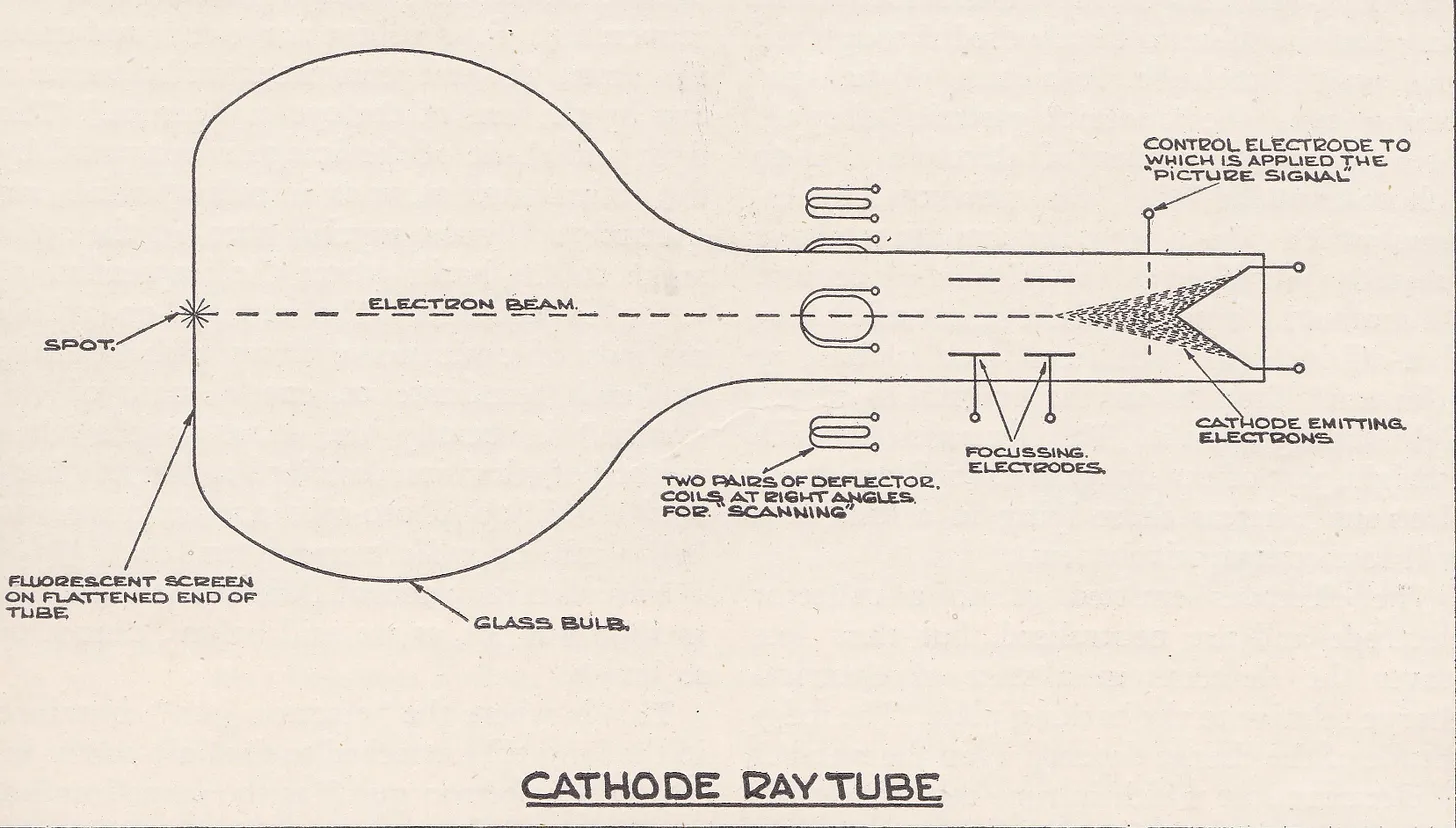
To tackle this, the lab hoped to recruit a graduate student to create a proof-of-concept for a high-speed oscilloscope, a device that could directly visualize electrical pulses. A cathode ray oscilloscope worked by firing a beam of electrons across a phosphorescent screen inside a vacuum tube, where the impact produced a bright spot of light. Electric fields could be used to deflect the beam horizontally (to represent time) and vertically (to represent signal amplitude) so that electrical signals appeared as moving lines of light that could be observed directly.
Although cathode ray oscilloscopes were already in use, they served mainly to capture slower signals. The high voltage surges experienced in thunderstorms or short circuiting events, though, flashed by in one hundred millionths of a second, leaving almost no trace on the screen. To make such fleeting signals visible, the intensity of the electron beam had to be increased, which meant focusing the beam into as small and powerful a spot as possible. Only one student applied to take on the challenge: 21-year-old Ernst Ruska.
Ruska was born into a family of scientists in Heidelberg, Germany, in 1906. He had been exposed to optics from an early age, as his uncle was an astronomer at the local observatory and his father, a science historian, owned a large optical microscope that Ruska was strictly forbidden to touch. He recalls in his Nobel lecture: “We would see on a table in the other room the pretty yellowish wooden box that housed my father’s big Zeiss microscope … He sometimes demonstrated to us interesting objects under the microscope, it is true; for good reasons, however, he feared that children’s hands would damage the objective or the specimen by clumsy manipulation of the coarse and line drive. Thus, our first relation to the value of microscopy was not solely positive.”
Unlike the rest of his family, Ruska’s passion leaned less toward science and more toward technical projects and problem-solving through engineering. While the other Ruska children spent their weekends with their father classifying rock samples or identifying bird calls, Ernst preferred tinkering with electrical switchboards and reading Max Eyth’s Behind Plow and Vice, a memoir on engineering and invention. And when he grew older, he recalls being fascinated by his high school physics teacher’s explanations of the movement of electrons through electrostatic fields and the limitations of light microscopes — an interest he carried into adulthood.
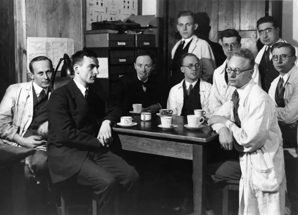
At the High Tension Laboratory, under Max Knoll, Ruska began building the much-anticipated oscilloscope. In this device, the incoming electrical current would pass through the vertical deflection plates, causing the electron beam to shift in proportion to the amplitude of the surge. To sharpen the image, a magnetic focusing coil was placed upstream of the deflection plates, concentrating the beam into a small, bright spot before it reached the phosphorescent screen. Ruska’s task was to determine the optimal placement of these coils so that the dot appeared as sharp as possible.
For guidance, Ruska turned to Hans Busch’s recent papers on the lens-like action of magnetic fields on electron beams. In these papers, Busch had not only shown that a coil could act as a “magnetic electron lens,” but had also worked out the formulas describing electron trajectories in such a field and how the focal length changed with coil current. Using these calculations, Ruska confirmed Busch’s theories experimentally and determined the precise coil placement needed to bring the beam to a sharp focus. He then placed a small aperture in the beam’s path and, by varying the coil current, was able to project and record an image of the aperture at different magnifications on a screen.
As Ruska later recalled in his Nobel lecture, his 1929 Master’s thesis contained “numerous sharp images with different magnifications of an electron-irradiated anode aperture … the first recorded electron-optical images.”
By 1930, as Germany’s economy collapsed under the weight of post-war reparations and global depression, Ruska was unable to find work in industry and remained at the university for doctoral studies. Initially unsure of a research direction, he continued experimenting with magnetic lenses. He reasoned that if one coil could produce a magnified image, two in sequence might enlarge it further — the conceptual birth of the electron microscope.
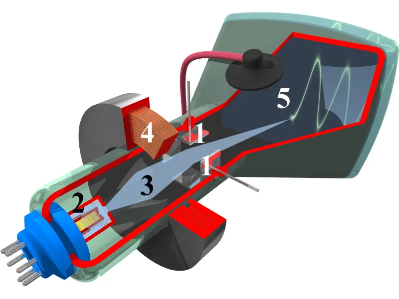
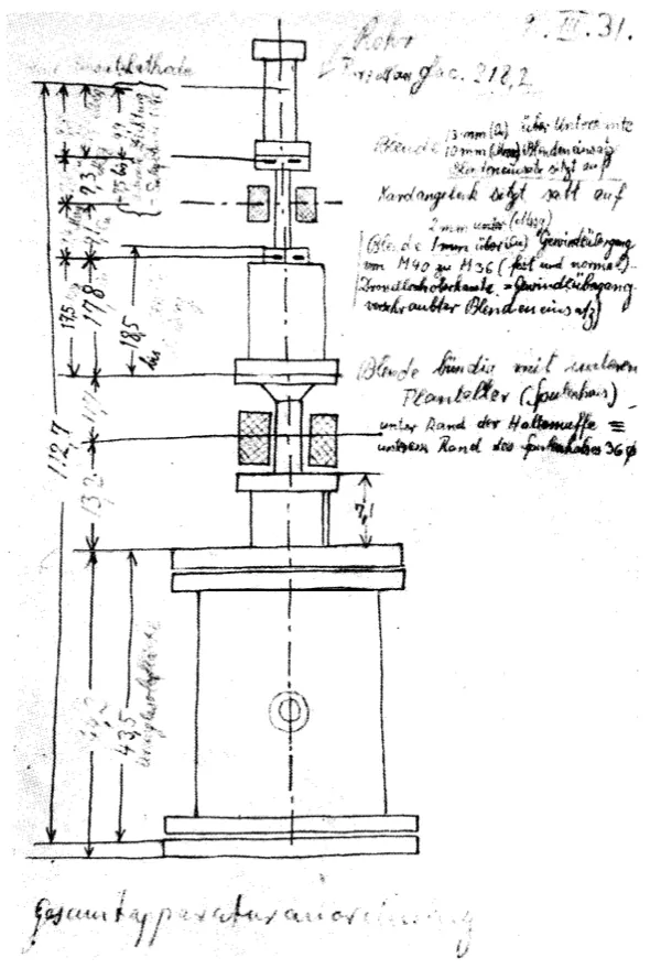
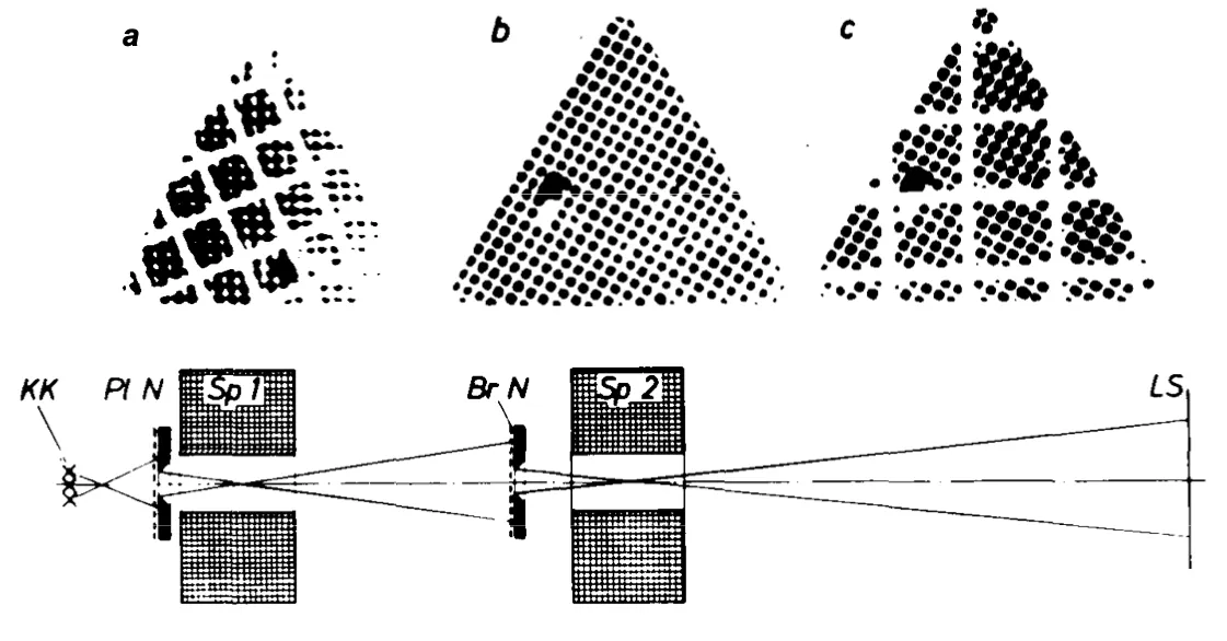
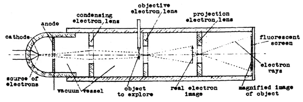
By April 1931, Ruska had constructed a two-stage imaging system with a total magnification of 14.4 times — still far below the roughly 1000-fold magnification achieved by high-quality light microscopes of the time. The system began with a cathode inside a vacuum tube, which emitted electrons when a high voltage was applied. These electrons were accelerated toward an anode and passed through a small aperture, forming a narrow beam, much like light through a pinhole. Magnetic coils wrapped around the tube acted as electron lenses. The first coil, placed close to the object, served as the objective lens, bringing the transmitted electrons into focus and forming an intermediate image. A second coil downstream acted as a projector lens, refocusing and enlarging that intermediate image so it could be captured onto a fluorescent screen.
By carefully tuning the currents in both coils, Ruska could control the focal lengths and achieve much higher magnifications than with a single lens. The final image appeared as glowing light patterns on the screen, with bright areas where electrons passed through the specimen and dark regions where they were absorbed or scattered.
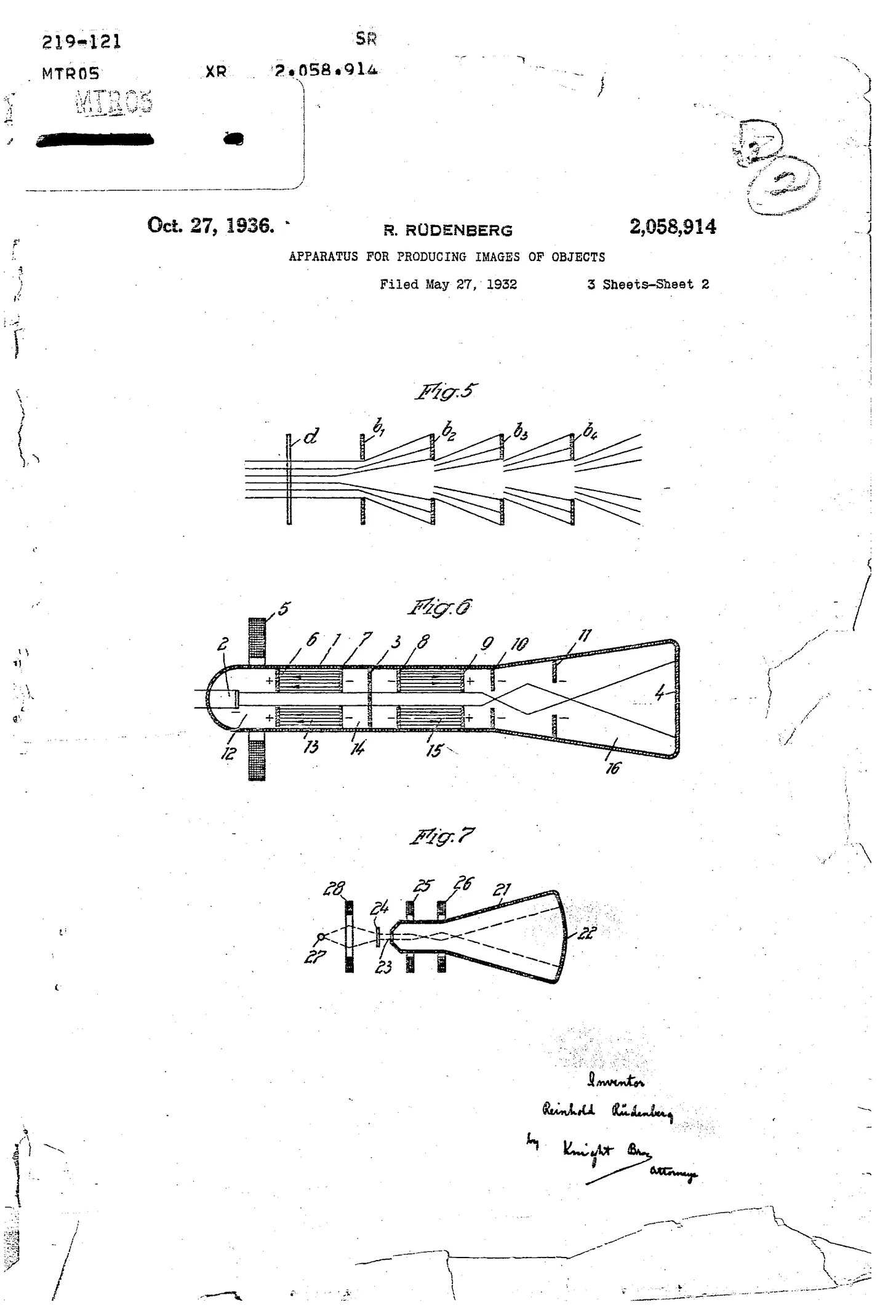
These images, photographed through a window in the tube, were the first electron micrographs, created by channeling electrons through successive magnetic lenses in a multistage system. Although its resolution was quite modest by today’s standards, this instrument is regarded as the first electron microscope. Ruska submitted the results for publication that same month, though the paper did not appear until August. Unfortunately, unbeknownst to him, between its submission and publication, a patent for an electron microscope had already been submitted by another inventor: Reinhold Rüdenberg.
Rüdenberg, born in Hanover in 1883, came of age during a golden decade of physics marked by Röntgen’s discovery of X-rays, the identification of the electron, and the first studies of radioactivity. As a high-school student, he eagerly replicated many of these experiments, building a two-way Morse telegraph, powering an X-ray tube with a hand-wound inductor, and constructing a radio transmitter and receiver. He received his first patent, for a radio oscillator, while still an electrical engineering student at the Technical University of Hanover.
After earning his doctorate, Rüdenberg spent three years (1906-1908) at Göttingen University, working in applied mechanics and collaborating with leading figures in electron theory, including Hans Busch. In 1908, he joined Siemens in Berlin as a design engineer and, by 1923, had risen to the position of Chief Electrical Engineer.
While at Siemens, Rüdenberg developed several new electrical designs, among which were cooling systems for high-voltage generators, one of the first 60-megawatt turbine generators, conductors for high-voltage transmission lines, and relay systems for distant power stations. He also spent three years apprenticing in Siemens’ patent department, an experience that doubtless helped fuel his prolific output of them. He was a prolific inventor and is estimated to have held over a hundred unique patents.
In the fall of 1930, while on vacation, Rüdenberg’s youngest son fell gravely ill. The three-year-old developed a high fever and paralysis. He had contracted polio. At a time when thousands were infected each year in Germany, with fatality rates around 15 percent, the diagnosis was devastating. Worse still, almost nothing was known about the “germ” responsible: No diagnostic test, no treatment, and no vaccine existed.
“This amazing fact and its significance for science and health gave me no rest in my thoughts,” Rüdenberg later recalled. “During many sleepless nights, tortured by the fate of my son, agonizing fantasies came and went, how to find ways to examine these minute germs, how possibly to attack them in order to attain healing or at least a standstill of the disease. Certainly, an agent finer than light had to be found to make these tiny viruses of immeasurable size visible to the human eye.”
Motivated by both paternal concern and engineering instinct, Rüdenberg began searching for a way to see such viruses. He considered X-rays but quickly dismissed them, as no method existed to focus the X-ray particles like visible light. Electrons, however, held promise. Having studied their behavior with Busch at Göttingen, he was aware of the focusing power of magnetic fields, and when Busch later published his 1926 and 1927 papers on magnetic electron lenses, he even sent copies directly to Rüdenberg.
During the winter of 1930-1931, Rüdenberg sketched out a complete conceptual design for an electron microscope, detailing its electron source, electrostatic lenses for focusing and magnification, and a fluorescent screen for visualization. In May 1931, just one week before Ruska publicly presented his own work, Rüdenberg submitted a series of patent applications describing this electron microscope.
Meanwhile, unaware of Rüdenberg’s patents, Ruska also pressed forward. For his doctoral research, Ruska focused on improving the electromagnetic lens, whose magnification ability still lagged far behind the optical lenses of conventional light microscopes. At the time, a state-of-the-art light microscope could magnify images up to about 1000 times, whereas in 1932, extant electron microscopes were still stuck at a paltry 17-fold.
To improve their performance, Ruska realized he needed to decrease the electron microscope’s focal length, since a shorter focal length would bend electrons more strongly, bringing them to a smaller focal point and producing a higher magnification. He discovered that encasing the coil in iron did so dramatically. This led to the invention of the polepiece lens, now a fundamental component of all electron microscopes.
Polepieces are shaped iron cylinders, each with a coil, placed a few millimeters apart. The narrow gap concentrates the magnetic field, producing a lens with stronger focusing ability and a shorter focal length. This not only increased the magnification but also provided more space to add a third lens (a condenser lens upstream of the sample) within the cathode ray column.
During this time, Ruska and Knoll also made a bold attempt to estimate the theoretical resolution limit of the electron microscope. They applied the formula used in light microscopy and substituted the wavelength of electrons for that of light. For electrons accelerated at 75 kilovolts (higher voltages would increase the electrons’ energy and further shorten their wavelength, which, in principle, yields even finer detail), they arrived at a resolution limit of 2.2 angstroms (2.2 x 10⁻¹⁰ meters).8
Ruska submitted his dissertation in mid-1933 and later that year built a vastly improved microscope, achieving magnification up to 12,000 times. The images, taken of a scrap of aluminum foil, exceeded the resolution limit of the light microscope for the first time (even though the high-energy beam incinerated the samples).
Ruska observed that very thin foils produced sharper images with stronger contrast while also surviving longer under the beam. He reasoned that, in thin specimens, most electrons passed through without losing energy, elastically scattered (diffracted) rather than absorbed. These transmitted electrons still carried structural information and built up the image on the screen. Because fewer electrons deposited energy in the material, less heating and radiation damage occurred, allowing longer exposures and finer detail.
By 1934, Ruska had published these findings and even speculated about imaging biological material. He stated, “This microscopy is accessible to any objects (including all organic ones), provided that they can be prepared as sufficiently thin foils and introduced into the vacuum without suffering damage (structural alteration).” And, “For better visualization of such objects — one might think, for example, of nerve fibrils with their extremely fine structure — it will perhaps be necessary to develop ‘staining’ methods adapted to the problem, such as impregnation with metal salts (silvering), similar to those already commonly used in ordinary histological microscopy.”
Rüdenberg’s design, meanwhile, was never built at Siemens. The political upheaval in Germany halted his advancement, as a German of Jewish descent, threatened his very survival. In 1936, with Siemens’ assistance, he and his family fled to England and, two years later, emigrated to the United States, where he became a professor of electrical engineering at Harvard.
Ironically, as a German, Rüdenberg was received with ambivalence; in 1942, during the war, his U.S. patents on the electron microscope were seized by the Alien Property Custodian, a government office tasked with seizing assets belonging to citizens of enemy nations during wartime. Post-war, he had to fight lengthy legal battles to reclaim them. He later consulted for Farrand Optical Company, a small company in New York which attempted to build an electrostatic microscope based on his patents, a venture which failed commercially. Happily, even as these obstacles abounded, his son made a full recovery from his polio.
By the early 1930s, electron microscopy had surpassed the resolving power of light microscopes, promising magnifications several orders of magnitude higher. Yet progress was uneven.
In Belgium, the Hungarian physicist Ladislaus Marton built his own instrument by 1932 and produced the first biological electron micrographs: images of the insectivorous plant Drosera intermedia and the blood-red bacterium, Serratia marcescens.
To make such delicate samples visible, Marton turned to osmium tetroxide, a heavy metal compound that binds strongly to cellular membranes. By coating thin sections of Drosera intermedia with osmium, he increased their ability to scatter electrons, resulting in clearer contrast in the final image. He also introduced an electronic shutter, a device that blocked the electron beam during focusing and opened only for the brief moment of exposure. This protected fragile specimens from unnecessary radiation damage while still allowing sharp images to be captured. For a time, it seemed Marton was leading the field.
Ruska, who had completed his PhD in 1933 and took a job in the television industry, returned to the field. He joined forces with Bodo von Borries, a longtime collaborator and future brother-in-law, to push the technology toward commercial viability. Between 1933 and 1935, they filed eight patents and canvassed a wide range of institutions for financial support. They approached the Kaiser Wilhelm Institute, the board of optical manufacturer Carl Zeiss, and even steel companies to see if they had any need for electron microscopes. While initial efforts with Zeiss seemed promising, they collapsed when Zeiss withdrew due to Siemens’s rights to Reinhold Rüdenberg’s earlier patents.
Despite these setbacks, interest in electron microscopy mounted. At the Technical School in Berlin, students modified Ruska’s prototypes to capture striking images of a fly’s leg hair magnified 25,000 times. To make the tissues more resistant to the beam, they used potassium dichromate, a fixative that coss-linked lipids and proteins in the tissue so it was less likely to collapse or vaporize. This fixative also increased scattering contrast, making fine details easier to discern.
Specimens were cooled to –17 °C, which reduced thermal motion and slowed the buildup of heat from inelastic electron collisions. Cooling didn’t prevent radiation damage, but it delayed it long enough for images to be recorded. These were early explorations of the cryogenic methods that would later define the field.
By 1936, electron microscopy centered around a highly active (albeit small) community with Marton in Belgium, Ruska and von Borries in Berlin, and younger researchers at their university extending the work. However, all still lacked financial support to develop a commercial system.
Momentum shifted when Ruska spoke at the 1936 German Conference of Physicists and Mathematicians. His brother Helmut, a physician newly appointed at Berlin’s University Hospital, added crucial medical endorsement by promoting the microscope’s potential in medical applications. This medical credibility brought Siemens back to the table. With both Siemens and Zeiss expressing interest, Ruska and von Borries chose Siemens, which already held the Rüdenberg patents and had stronger electrotechnical expertise.
In February 1937, a decade after Hans Busch first theorized the electron lens, Siemens launched development of the first commercial electron microscope in Berlin. By 1938, the first model was available, offering magnification of up to 30,000 times.
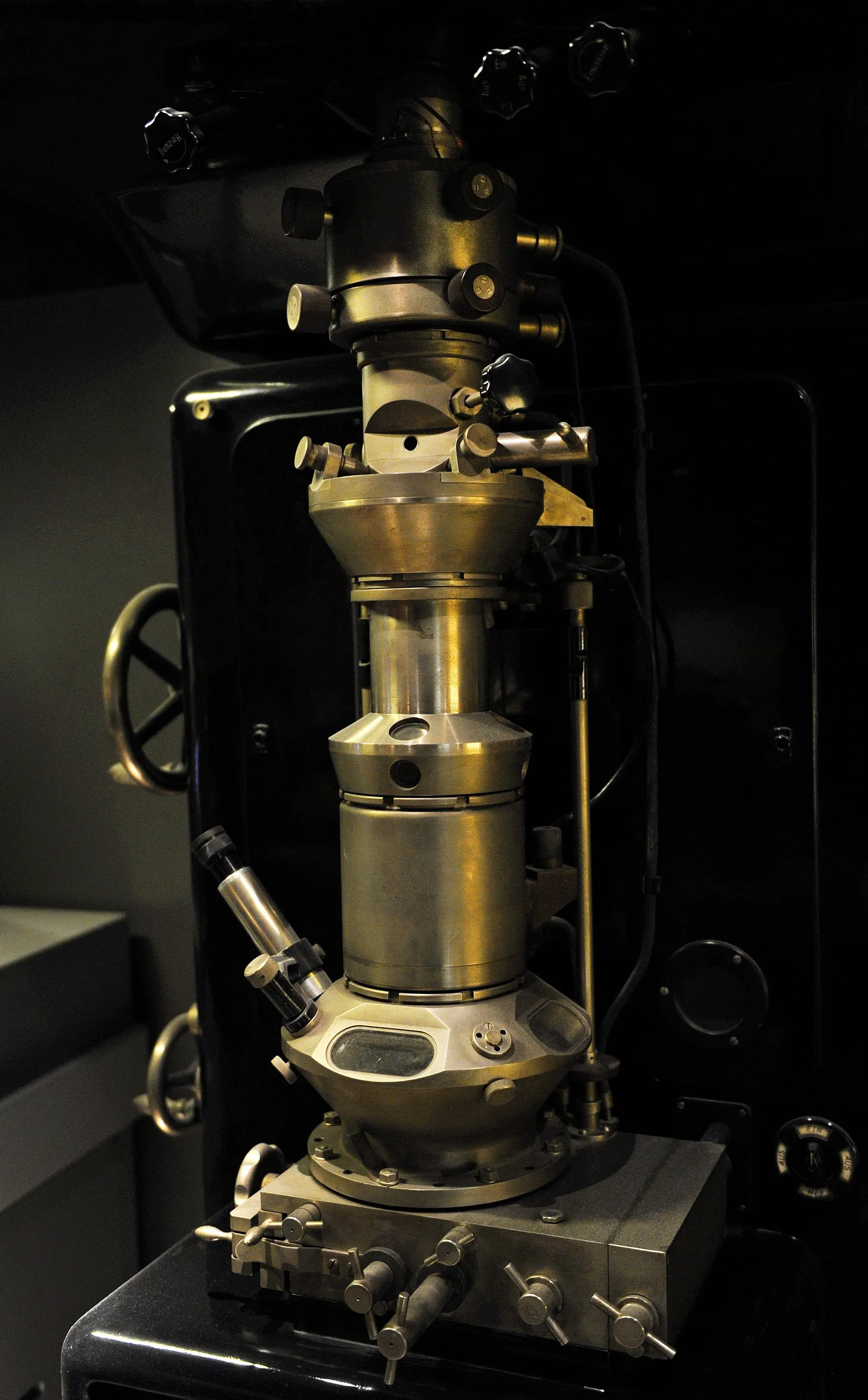
The device was a triumph of Ruska’s bench-top experiments and relentless iteration. At the top of the microscope column sat the cathode, generating electrons accelerated downward at high voltage. A condenser lens collected, narrowed, and focused the electron beam to illuminate the sample, which was introduced through a small vacuum airlock and held on a stage. Immediately below it lay the objective lens, a powerful magnetic coil that brought the transmitted electrons into sharp focus, forming a first, intermediate image. A second coil, the projection lens, then enlarged this image and cast it onto a fluorescent screen, where bright and dark regions revealed the specimen’s structure. Researchers could view the glowing picture directly through a built-in window or capture it on photographic plates housed beneath the screen. To maintain stable operation, the entire column was kept under high vacuum by a mercury diffusion pump.
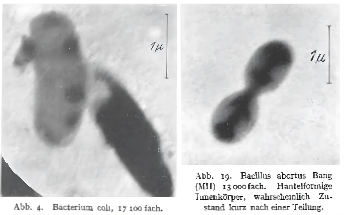
A shared Siemens laboratory was set up and became an important hub for producing some of the earliest biological electron micrographs. Directed by Helmut Ruska, it housed four instruments available to visiting scientists, many of them biologists and medical researchers. In 1939 alone, nearly 2,000 images were produced, leading to 23 publications. Among them were the first electron micrographs of viruses, bacteriophages, and fine biological details never before seen.
The lab itself was destroyed in an air raid in 1944, and it would take nearly a decade before Siemens in Germany regained its footing in electron microscopy. But by then, the electron microscopy spark had spread: Laboratories in Britain and the United States continued to drive the field forward, building on the groundwork laid in Berlin. Ernst Ruska would go on to win the Nobel Prize in Physics in 1986 for his fundamental work in electron optics and microscopy.
Nearly a century after its invention, the electron microscope has transformed from a tool barely capable of resolving fuzzy virus particles into one capable of capturing atomic detail. While its progress has mostly been marked by steady refinements, it has also been punctuated by key breakthroughs.
For instance, from the start, electron microscopy for biology faced a water problem. Because the microscope operates under high vacuum, liquid water evaporates instantly, leaving delicate biological samples collapsed or distorted. To avoid this, aqueous samples had to be dried, fixed, or stained, which produced recognizable images but with obvious artifacts, such as shrunken cells, ruptured membranes, and structural distortions that no longer reflected the living state. Through the 1940s and 1950s, embedding samples in resins and the use of ultra-thin sectioning made cellular ultrastructure visible, while freeze-drying and early cryogenic sectioning offered partial preservation of hydrated material, though the results were still plagued by distortion.
A breakthrough came in the early 1980s, when Jacques Dubochet and his colleagues at the European Molecular Biology Laboratory in Heidelberg demonstrated that water could be vitrified; that is, cooled so rapidly that it solidifies into glass rather than crystallizing, finally allowing biomolecules to be preserved and imaged as they are in life.
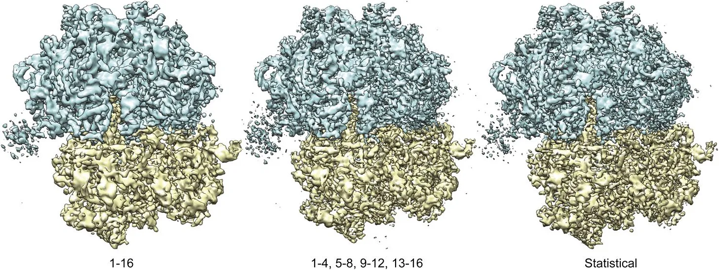
In parallel, computational techniques were improving. Beginning in the 1970s, Joachim Frank developed statistical methods for aligning and averaging thousands of noisy electron micrographs of individual macromolecules. This “single-particle analysis” transformed faint, low-contrast images into coherent 3D reconstructions. When combined with Dubochet’s vitrification method, the two advances gave rise to single-particle cryo-electron microscopy: Molecules suspended in vitreous ice could be imaged in random orientations and computationally combined into detailed three-dimensional structures.
Three decades later, with the arrival of direct electron detectors, developed with the efforts of Richard Henderson and with more powerful algorithms, single-particle cryo-EM entered its “resolution revolution,” routinely delivering near-atomic detail and firmly establishing itself as one of the central methods of structural biology.
Today’s most advanced cryo-electron microscopes stand nearly two stories tall, cost millions of dollars, and operate with breathtaking precision. But they still rest on the same foundation laid in the 1930s: a beam of electrons, shaped by magnetic fields, interacting with matter to reveal what light cannot.
At the top of the vertical column is the electron gun, the source of the beam. A fine tungsten filament or sharp field-emission tip is held at high negative voltage, often 200–300 kilovolts, so electrons are released and accelerated down the column. At these energies, electrons travel close to the speed of light, with wavelengths thousands of times shorter than visible light, giving them their extraordinary resolving power. To prevent scattering, the column is maintained in an ultra-high vacuum, as even trace gases could deflect or scatter the beam.
Magnetic lenses, made of coiled wire encased in iron polepieces, focus and steer the electrons much like glass lenses bend light. The condenser lens narrows the beam onto the sample, while the objective lens forms the first magnified image. Additional projector lenses enlarge this image and deliver it to a detector.
When the beam passes through the specimen, electrons interact with its atoms. Some scatter elastically, shifting phase without losing energy; others scatter inelastically, losing energy, and are either absorbed or filtered out. The transmitted electrons carry structural information, encoded as variations in amplitude and phase, and create a contrast image on the detector.
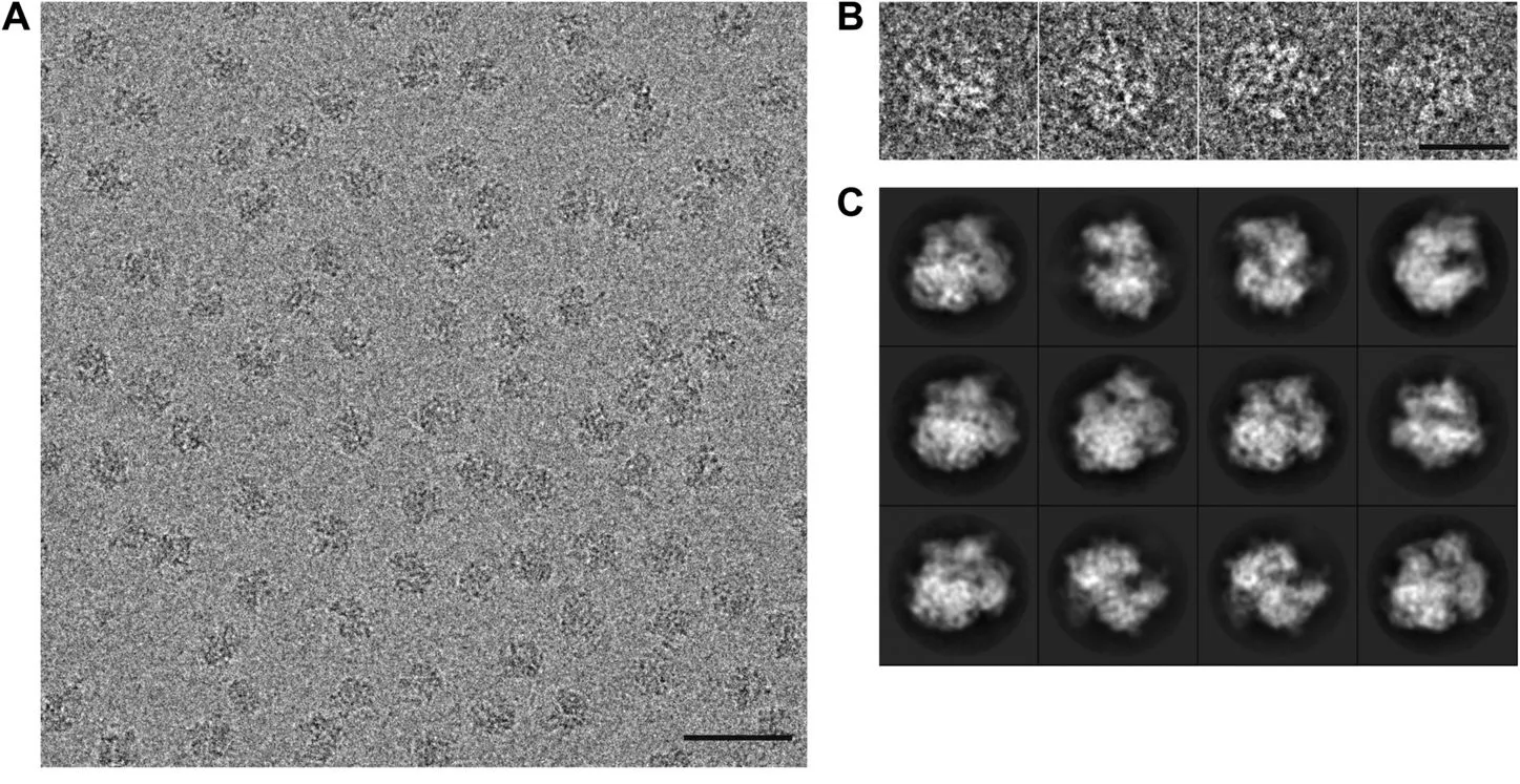
In cryo-EM, millions of such low-contrast 2D projections are collected, each a noisy snapshot of a molecule in a random orientation. Computational algorithms align, classify, and combine them, using a mathematical method that breaks the images down into their underlying patterns of waves (using the Fourier transform), then piece those patterns back together to form a detailed 3D map.
The result begins as a grainy micrograph, but when assembled and refined, this picture reveals extraordinary detail: the honeycomb lattice of graphene, the folds of a viral capsid, or the ribosome caught mid-translation.
Today, no single imaging method captures everything. For following fast processes, tracking molecules in living cells, or imaging whole organisms, light microscopy remains indispensable. For atomic resolution of well-ordered proteins, X-ray crystallography is still unmatched.
But when it comes to bridging the scales between atoms and cells, there is no better tool than the electron microscope. The same instrument that in 1938 revealed the faint silhouettes of mouse ectromelia virus now resolves viral proteins at the scale of a chemical bond, an arc of progress that has helped biologists redefine what it means to “see.”
{{divider}}
Smrithi Sunil is a research scientist developing imaging techniques to study how the brain works across scales. She has developed multimodal microscopy methods to bridge molecular, cellular, and systems-level measurements of structure and function. She also writes about science and metascience on her Substack, Engineering Discovery.
Thanks to Nicholas Porter and Alicia Botes for reading a draft of this essay. Lead image by Ella Watkins-Dulaney, adapted from Vossman/Wikimedia and Ernst Ruska. Whole-cell animation and video by Martina Maritan, Scripps Research.
Cite: Sunil, S. “Making the Electron Microscope.” Asimov Press (2025). https://doi.org/10.62211/57hg-22fw