Over the past few months, AI-based tools have emerged that enable scientists to design original antibodies on the computer for the first time. A year ago, none could reliably do this computationally. But now companies like Nabla Bio, Chai Discovery, Latent Labs and, most recently, DeepMind-spinoff Isomorphic Labs have allowed high success rates. There are even open source tools, such as BoltzGen and Germinal, that deliver similar performance.

The rapid progress in antibody design matters because these molecules are among the most versatile tools in biology. Many medicines — including Humira and Adalimumab — are antibodies, and cheap diagnostics, including $1 COVID tests, rely on them as well. These Y-shaped proteins make excellent binders, as the two arms can latch onto proteins or other molecules and block their activity.

Before these AI tools existed, scientists searching for a useful antibody would first need to screen billions of candidates in laboratory assays to identify just a handful with high affinity for a target. BindCraft, released in 2024, changed this. For many targets, a suitable binder can now be found after just tens of attempts rather than billions. BindCraft uses the AlphaFold 2 model, but inverts it: the model creates a protein structure expected to fit onto a chosen target, then converts that “shape” back into an amino acid sequence that can be synthesized and tested in the laboratory.

Antibodies are not the only type of protein binder, and binders are generally catalogued according to their size. A “peptide” is any protein smaller than 30 amino acids, a “mini-binder” is between 50 and 250 amino acids in size, and an “antibody” covers anything from a 120-amino-acid antibody fragment to a multi-chain, 1,300 amino acid molecule.

Computational drug developers spend most of their time designing a particular type of antibody fragment, called the VHH, or “nanobody.” These are small variants of antibodies, naturally produced by llamas and alpacas, consisting of a single heavy chain. VHHs are much easier to design than a full antibody because they are about one-tenth the size and more compact. They can also be cloned and expressed in bacteria, unlike full antibodies, which require glycosylation, a chemical modification that only yeasts and mammalian cells can perform.

The main goal in binder design is to find a molecule with a high affinity to some target, meaning the binder latches on tightly and won’t let go. Such affinity is quantified by a dissociation constant, or Kd, which describes the concentration of free binder that must be present for a target molecule to have a 50 percent chance of being bound. A lower Kd means tighter binding. Picomolar (pM) and nanomolar (nM) Kds are typical for drugs, while micromolar (µM) is considered quite weak.

Semaglutide, for example, binds its target with sub-nanomolar affinity, while many natural signaling proteins, like T-cell receptors, have affinities in the micromolar range; a thousand-fold weaker. In the binder-design literature, a sub-micromolar affinity is often used as the threshold for calling a design “successful,” though this affinity would likely not be strong enough to be therapeutically useful.

To learn antibody design, most people start with BoltzGen, a tool developed by Hannes Stärk and the team at Boltz. (This is the same team behind Boltz-2, one of the leading AlphaFold 3-like structure prediction models.) BoltzGen is, arguably, the leading open-source approach for computational antibody design, and unlike many competitors, it uses the permissive MIT license, meaning anyone can use it, even commercially.

Working with multiple academic labs, the Boltz team showed that BoltzGen achieves sub-micromolar binders in a majority of cases, on both well-studied proteins like insulin and on difficult targets with no known similar structures. That said, BoltzGen is not the only option, and the landscape is shifting quickly. RFantibody can design full antibodies rather than just fragments, and Mosaic allows users to incorporate custom scoring functions.

However, none of these tools are easy to use. Designing an antibody on the computer requires navigating a huge tangle of jargon, a general understanding of the pros and cons of available software tools, and enough familiarity with wet-lab biology to know what to do after the design process has been completed. This guide walks readers through the full process of designing an antibody from home using BoltzGen.

{{signup}}

The computational process involves five steps: choosing a target, preparing its structure, running a design campaign, filtering candidates, and experimentally validating the results. The guide follows a single hypothetical candidate and describes each step using the best open-source tools currently available.

1. Choosing a Target

This guide will use Nipah virus Glycoprotein G — “Nipah G” — as its protein target. Nipah G sits on the surface of the virus, a dangerous pathogen with a mortality rate of between 40 and 75 percent, and is essential for binding human cells. A binder that blocked Nipah G would presumably help prevent infection. (One antibody, m102.4, has already completed Phase I clinical trials on exactly this basis.)

Nipah G was also the subject of a recent binder design competition hosted by Adaptyv Bio, a cloud lab for protein designers. These competitions matter because they pit design tools against one another, chasing the same target under identical conditions. The Nipah G competition attracted a few hundred entrants, including the BindCraft developer, Martin Pacesa, and the Mosaic developer, Nick Boyd. Adaptyv screened more than 10,000 designs in total, making this arguably the richest publicly available dataset for comparing binder design tools to date.

This guide’s main tool, BoltzGen, did not fare well. In fact, only one percent of designs passed the experimental binding threshold. The reason for this is unclear, but every protein target behaves differently, and no tool excels across all of them. While Mosaic had the best results of any tool in the competition, with 8 out of 9 designs successfully binding the target, it requires more hands-on coding and is better suited for those already comfortable with protein design pipelines.

2. Preparing the Target Structure

Choosing a target protein is only the first step; you also need to choose a specific crystal structure to work with. A single protein can have hundreds of structures in the Protein Data Bank (PDB), each produced under different experimental conditions, with small but consequential differences in atomic positions.

Proteins also shift shape depending on their state. A protein bound to another molecule looks different from one floating freely in solution. These two forms, called the holo and apo forms, respectively, can have entirely different geometries.

The PDB is the main repository for protein structures, but its search engine is imprecise. Querying “Nipah virus Glycoprotein G” returns 32 results, many unrelated to Nipah, and the interface is hard to navigate unless you are a crystallographer.

A better repository is UniProt. If you search for your target protein there, you will find that the UniProt team has already done the hard work of linking every relevant PDB entry to each protein it contains. The entries, however, vary as to what resolution they have, which protein chains are included, and even how much of the protein is physically present in the structure. It is not uncommon for a crystal structure to cover only part of the full protein. In the case of Nipah G, the available structures cover positions 176-602. This excludes the transmembrane domain of the protein, since that region is notoriously difficult to crystallize.

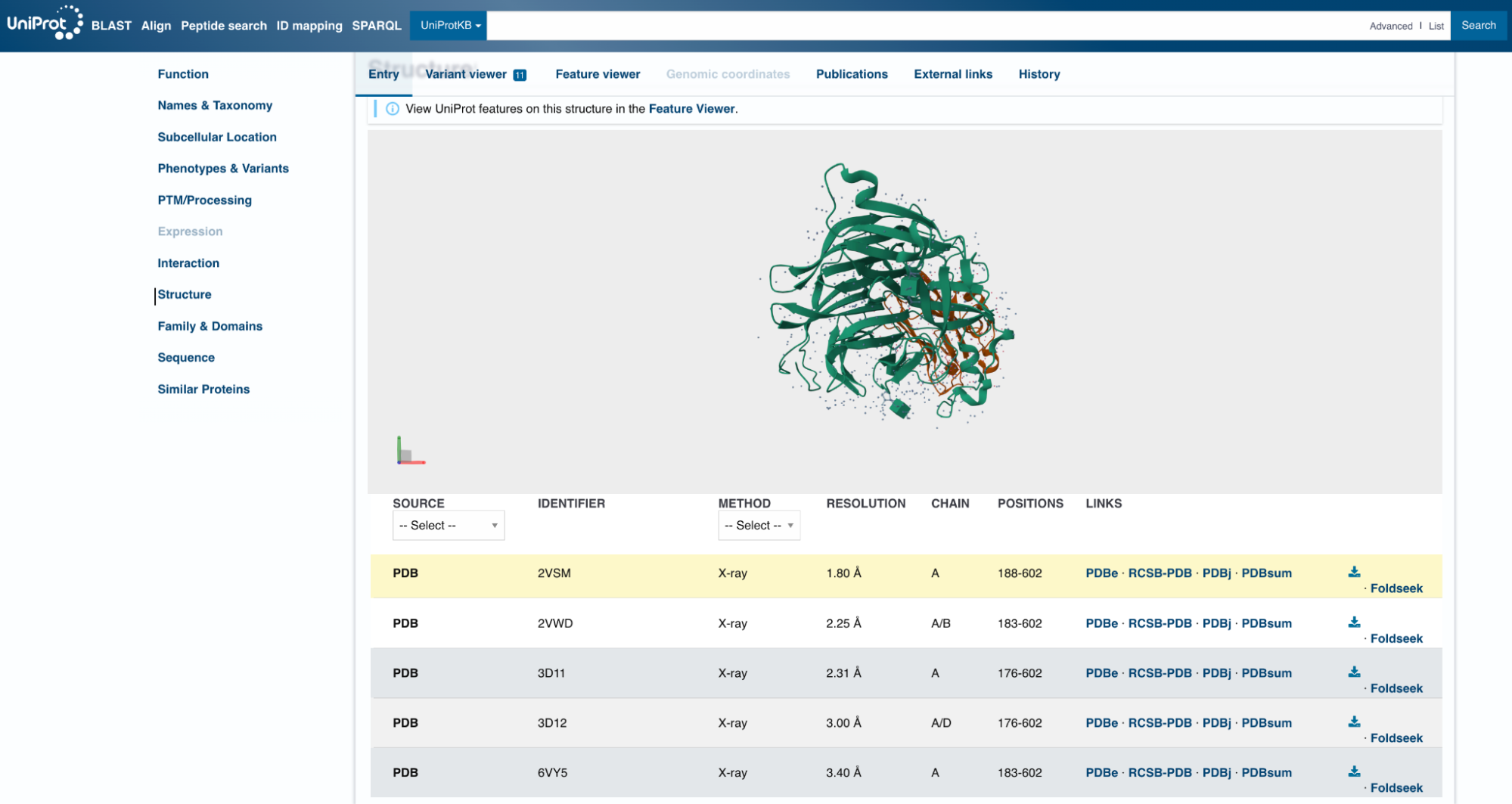
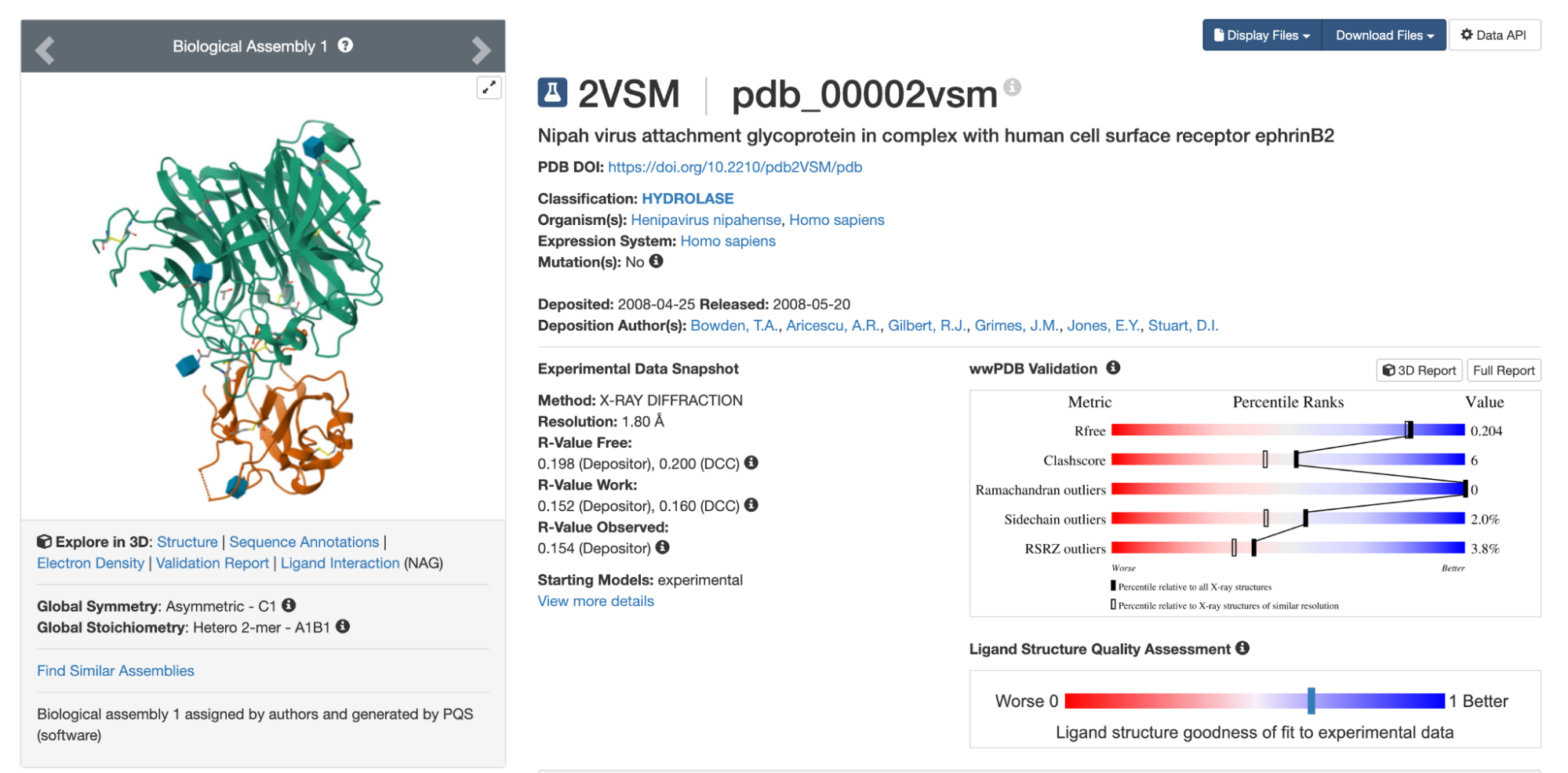
Looking at the UniProt list, 2VSM seems like a reasonable choice of target. It has the highest resolution of the available options, at 1.8 Å, slightly longer than a carbon-carbon bond. (Anything below 2 Å is considered high resolution for X-ray crystal structures.) The 2VSM structure also includes the virus’s natural receptor, Ephrin-B2, which shows exactly where on the surface a binder might attach.

Once you have a possible target, see what prior research exists. In this case, there is a 2025 paper that identifies binding sites (or “hotspots”) on Nipah G suited to binder design. The first hotspot is located at residues Q559, E579, I580, Y581, and I588, exactly where the virus contacts Ephrin-B2 and where the clinical antibody m102.4 binds. The second site — at residues V235, S236, Y237, R555, and S586 — sits on another face of the protein. Antibodies that bind there do not block receptor attachment directly but prevent the virus from undergoing the conformational changes needed to enter a cell. The third site, formed by W504, F458, and L305, helps to stabilize the receptor-binding domain.

Even though 2VSM seems like a promising structure, it is still worth testing several options before committing. Small differences in atomic positions can affect the designs you get, and nearly identical structures sometimes yield distinct results for reasons that are not obvious in advance.

Predicting a Structure

When preparing the target structure, it’s important to remember that some proteins have no crystal structure in the PDB. UniProt often links to predicted structures directly, but if nothing suitable turns up, you will need to predict one yourself. For non-commercial projects, the best tool for this is AlphaFold 3.

AlphaFold 3 is straightforward to use. Log into alphafoldserver.com, enter your protein sequence, and wait a few minutes. You do not need to set any parameters. The output is a 3D view of the predicted structure and a downloadable .cif file, which is a modern version of the older .pdb format.

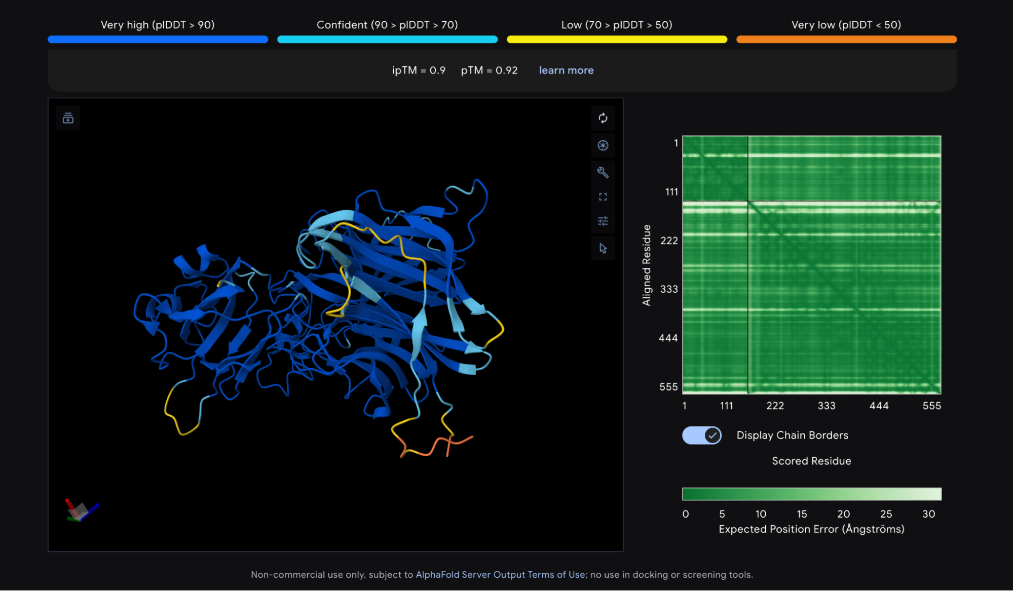
Protein structure prediction tools output a few different scores, or “confidence metrics,” though two come up most often. The first is pLDDT, which measures overall confidence in the predicted structure on a scale of 0 to 100. The second is ipTM, which measures confidence in the relative positions of two proteins in a complex, scored from 0 to 1. The Nipah G competition used a third metric, ipSAE, which is derived from ipTM and highly correlated with it, but tuned to better predict whether two proteins actually bind.

The AlphaFold 3 prediction for Nipah G bound to Ephrin-B2 looks good. Most of the structure shows a pLDDT above 90, the threshold for high confidence, and the ipTM is 0.9, meaning the model is confident about how Ephrin-B2 sits against Nipah G. The N and C termini score lower, but that is normal — those regions are disordered by nature. As a rule of thumb, a pLDDT above 90 and an ipTM above 0.8 are both good signs. This structure meets both of those cutoffs.

Trimming

Once you decide on a structure, it is often worth trimming it — that entails removing the parts of the protein irrelevant to the binding site. The cost of a design campaign scales roughly linearly with the combined length of the binder and target, so trimming irrelevant regions can save thousands of dollars.

The standard tool for this is PyMOL, a program for visualizing and manipulating protein structures. The open-source version can be installed via Conda, while the commercial version is available at pymol.org. Here are the specific steps you can take, using PyMol, to trim your target protein:

• First, load the 2VSM.cif file into PyMOL by typing fetch 2VSM or clicking File / Open and selecting the downloaded file. This loads the complete complex, including Ephrin-B2.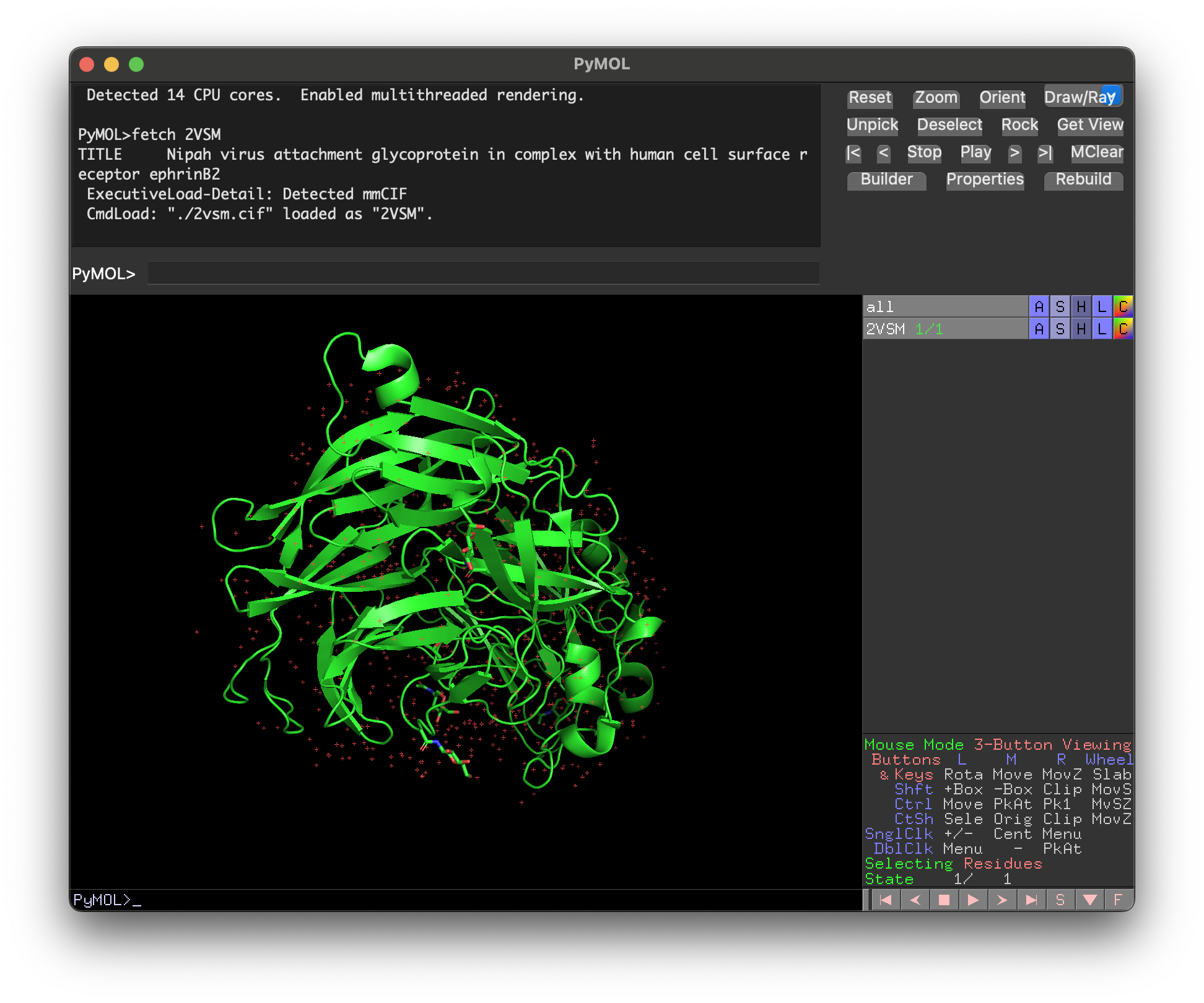

• To remove everything except Nipah G (chain A), type remove not chain A. To also show the protein sequence, type set seq_view, on. The red dots on the screen are mostly water atoms, which can be removed with the command remove hetatm.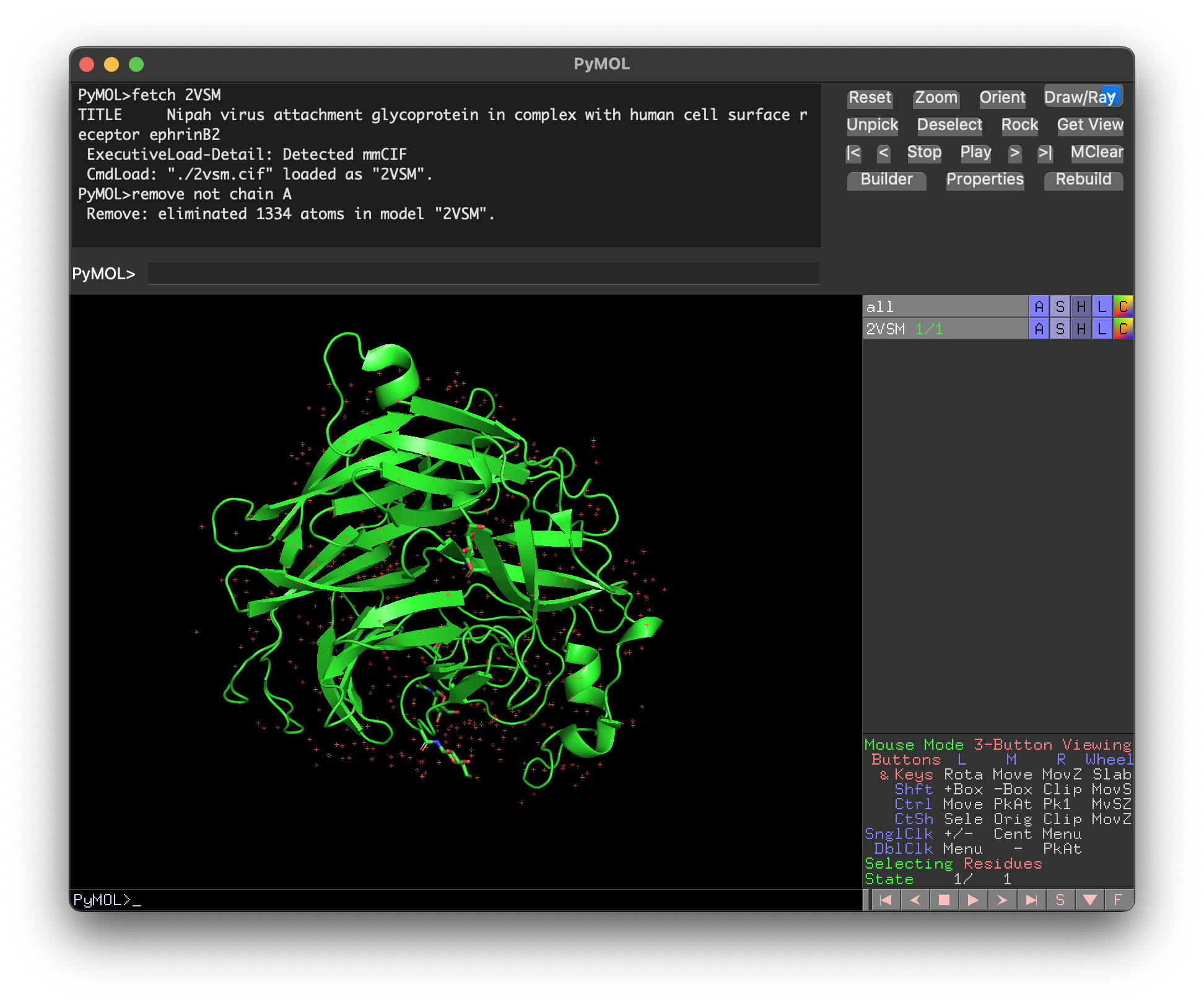

• Select and color the first hotspot with select hotspot1, chain A and resi 559+579+580+581+588; color red, hotspot1 so you can see where it is. Then, manually select residues (pink dots) by highlighting the sequence (here, I have selected positions 188 to 207.) Every amino acid after position 207 is quite close to the hotspot residues, so they cannot be safely removed.

• Finally, remove the sequence with the command remove resi 188-207 and save the edited structure with save 2VSM_trimmed.cifand save 2VSM_trimmed.pdb. (It is often useful to have both .cif and .pdb files.)

In this particular case, removing 20 amino acids from a 400 amino acid structure is hardly worth the effort, since the Nipah G hotspot sits close to both ends of the protein. Residues can also be removed from the middle of a structure, creating gaps, though this requires more testing. Gaps can cause problems with structure prediction and change the numbering of hotspot residues in BoltzGen. For large antibody design campaigns, however, trimming as aggressively as possible is usually worth the effort.

3. Running a Design Campaign on Ariax

BoltzGen is not easy to run locally. Your options are cloning the GitHub repository and running it yourself, using a cloud service like Modal, or working through platforms like Tamarind Bio, Litefold, or Neurosnap. The BoltzGen team also recently launched their own platform, Boltz Lab, currently in beta.

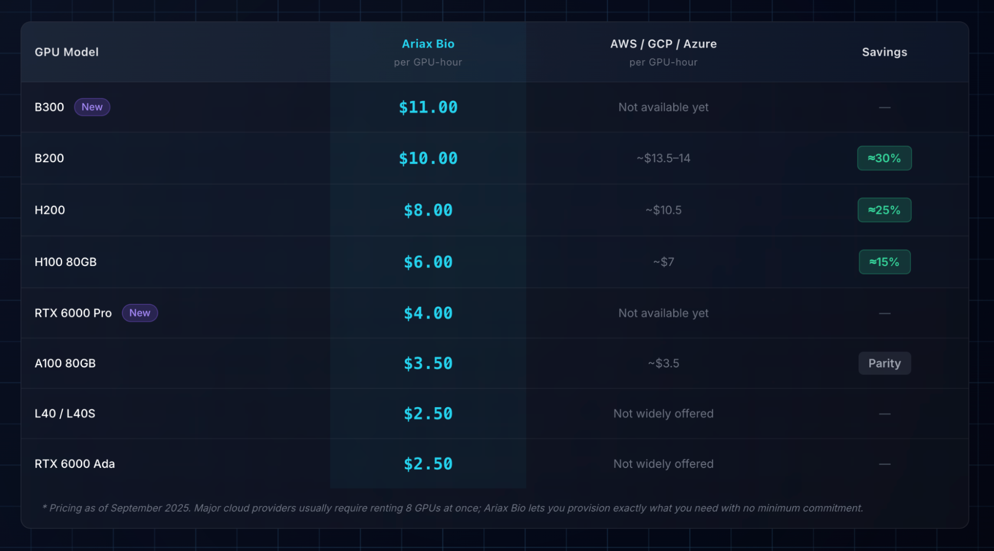
This guide uses a web-based tool called Ariax, arguably the easiest way to run BoltzGen and BindCraft. Ariax charges directly for GPU time, without the need for a subscription, and the team behind it are protein-design experts whose explicit goal is to make binder design easier.

Start small and run short campaigns with 100 or fewer designs for each of your candidate hotspots first. This will give you a sense of which one looks most promising. Once you have identified the best hotspot, scale up to a full campaign — roughly 50,000 designs. (The right number depends on the difficulty of your target, your budget, and how many high-scoring designs you need. More designs means a higher chance of finding something that works.)

Setting up a run on Ariax takes only a few minutes. The Ariax team have written a helpful tutorial with additional tips, and the defaults are sensible enough for both beginners and experienced users, though not every BoltzGen parameter is exposed. If you wanted to use a custom VHH framework, for example, you would need to generate the appropriate configuration files and run BoltzGen yourself. The BoltzGen documentation covers this, though getting GPU-dependent tools like BoltzGen running locally can be genuinely challenging.

To run a Nipah G campaign on Ariax, follow these steps:

1. Select VHH as the design scaffold, then upload the 2VSM_trimmed.pdb file created earlier. Although .cif files have largely replaced .pdb as the standard format, .pdb is still the safer choice here as .cif files exported from PyMOL are not always compatible with BoltzGen. If you need to convert between the two formats, use maxit, a conversion tool maintained by the PDB team.
2. Under Binding Rules, set “binding” to positions 349, 369, 370, 371, and 378. Note that these are not the original residue numbers, and this is an awkward but persistent problem with both .pdb and .cif files. After trimming, the 2VSM structure starts at position 211, but BoltzGen always counts from position 1. Ariax helpfully notes in its log that it has applied an index shift of -210, so to match BoltzGen’s numbering to the original, subtract 210 from each residue number. Visually check the hotspot positions in Ariax, which highlights them in yellow, to confirm they land on the expected residues.
3. You can optionally set “not_binding” positions to steer the design away from parts of the protein you want to avoid — glycosylation sites, for example, or regions far from the binding interface. This option is most useful for larger proteins with multiple domains; for Nipah G, the binders tend to land close to the target site without much guidance.
4. Set the # Designs to 50 and the Budget to 50. This just means you want to generate 50 designs, and return information for all of them. At this stage, it’s important to see the full distribution of scores across all designs, rather than just the top hits. But for the full campaign, when you scale up # Designs to 50,000, you’ll set the Budget at 100 or below to get back just the top scoring designs.
5. For GPU Selection, Cost or Performance mode both work fine for a small run. The only obstacle that can arise is if the protein is too large to fit in the GPU’s memory — for proteins above 400 amino acids, only the latest GPUs, such as the B200 and H200, may be able to handle it. For the full campaign, select Turbo Mode to run multiple GPUs in parallel (otherwise, the run can take days.) There is no real cost penalty for Turbo Mode, and the faster premium GPUs are not necessarily more expensive overall since they finish sooner.
6. Finally, click Validate Settings to check for errors, then click Start BoltzGen.

Before the campaign starts, you will also need to fund your Ariax account. Generating the 100 Nipah G test designs costs around $10. A full 50,000-design run would cost roughly $3,000-$6,000 for a protein of this size, since Nipah G is around 400 amino acids in length. The main way to lower costs is to trim the structure further. (Remember, though, that any time you remove part of the protein, you risk subtly altering its shape.) You also need to keep track of how the residue numbering shifts as a result.

Scoring

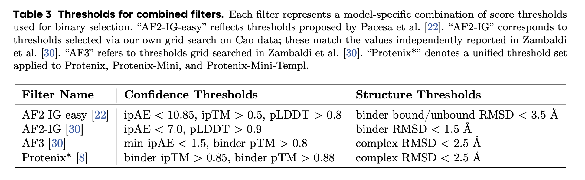
Scoring and ranking designs is one of the most involved — and most confusing — parts of binder design. BoltzGen outputs many metrics, including ipTM, predicted hydrogen bonds, and surface accessibility, combining them into a single “Quality Score” using a heuristic formula. The team behind PXDesign did a comprehensive review of scoring across BindCraft and other tools, and landed on thresholds of ipTM > 0.85, pTM > 0.8, and complex RMSD < 2.5Å as a reasonable way to separate binders from non-binders. These thresholds work fairly well, though as far as anyone can tell, no single metric or combination of metrics reliably predicts affinity.

There is no consensus on the best way to score designs. ipTM is a far-from-perfect predictor of binding, but it is a robust enough metric for comparing designs across hotspots. Previous Adaptyv Bio competitions ranked designs by ipTM, and although the latest competition used ipSAE instead, the two scores are highly correlated. For our Nipah G example, the differences between hotspots are large enough to be genuinely informative; the first hotspot — the Ephrin-B2 contact site — seems to be best, with an average ipTM of 0.68, compared to 0.56 for the third hotspot and 0.4 for the second.

You can also run BoltzGen without specifying a hotspot at all, letting the model find its own binding site. This approach worked remarkably well for Mosaic in the Nipah G competition, and Nick Boyd discusses it in more detail on the Escalante blog.

For the full campaign, it is worth starting with around 1,000 designs to check the cost per design and confirm that the designed binders look sensible. If the top designs from that first batch are not engaging with the intended hotspot, something has gone wrong; adding “not_binding” residues can help steer the model away from wherever it is mistakenly landing. Once everything looks reasonable, scaling up is easy. On Ariax, just click “Clone & Reuse,” adjust the number of designs to 50,000, and start the run.

4. Filtering and Selecting Candidates

For this example, the campaign ran to 1,000 designs. But the process for evaluating the top designs is the same regardless of how many you generate.

The best binder from this run, ranked by BoltzGen’s heuristic score, has an ipTM of 0.78. ipTM is not an intrinsic property of the binder itself, but a metric of Boltz-2’s confidence in the predicted binding pose. A different model, generating exactly the same binder design, might give a different score for the same metric.

AlphaFold 3 is generally thought to be the best structure prediction model overall and especially strong with antibodies and nanobodies. For greater confidence, you can run the same binder design through alphafoldserver.com as an independent check. A “good” design will typically get good ipTMs from both Boltz-2 and AlphaFold 3.

In PyMOL, load both .cif files, align them, and compare the BoltzGen pose to the AlphaFold 3 pose against the Nipah G structure. Since Nipah G is in the PDB, both structures should align closely. In this case, BoltzGen gives the design an ipTM of 0.78, while AlphaFold 3 gives its slightly different pose an ipTM of 0.73.

Several things about this design are worth noting. First, the Boltz and AlphaFold 3 poses are very similar. (If the two models had predicted different binding poses, the design should probably be rejected.) Second, the binding pose is next to the hotspot, and binding appears to be driven by the VHH’s hypervariable regions (called “CDRs”). It is not uncommon to have designs where, instead, the VHH binds “side-on.” This is not necessarily a bad thing, but it reduces the probability that it is a specific binder, only binding to the Nipah G target.

Third, the ipTM scores seem reasonable. It would be better if both were above 0.8 or even 0.9, but 0.73 is a decent ipTM from AlphaFold 3. And finally, the amino acid sequence for the designed binder looks plausible. Sometimes, binder design tools will output suspiciously low complexity sequences, like long runs of glycines or glutamates.

Computationally-designed proteins may also contain stretches of cysteines, which are likely to cause aggregation or clumping. A more thorough check would involve running the sequence through an antibody language model like AbLang, which scores how “antibody-like” a sequence looks.

On balance, this design does not score especially highly, but it may still be worth testing. Further computational tests could be done, though the returns diminish quickly. The only way to know whether a design actually binds is to test it in the lab.

5. Experimentally Validating the Results

Once you have selected your most promising designs, the next step is to test them in the lab. Almost everyone working in protein design uses Adaptyv Bio for this — the same group that ran the Nipah G competition. Adaptyv is a modern contract research organization, which in practice means you can go online, submit a list of protein sequences, and pay by credit card without a sales call. Adaptyv makes a small quantity of each design in a cell-free system and returns binding affinity data against your target in a few weeks. It is the closest thing available today to a true cloud lab.

Each design costs $119-215 to test, depending on how many you submit. Assuming a full campaign of 50,000 designs and testing the top 50, the total comes to roughly $4,000 for compute and $12,000 for testing — plus a few hundred dollars for Adaptyv to acquire the target protein. Careful filtering before submission can reduce these figures.

Published results from groups like Nabla Bio, Chai Discovery, Latent Labs, BoltzGen, Germinal, and mBER suggest binder design success rates (defined as finding at least one sub-micromolar binder from ten tested designs) of up to 66 percent. But the messy reality, based on wet-lab testing, is that the true number is probably far lower.

The most comprehensive dataset available for a single target binder is the Nipah G competition, where the success rate was under 10 percent. Mini-binders appear to be easier to design computationally than VHHs and, anecdotally, the success rate for tools like BindCraft and PXDesign across a range of proteins is probably a bit above 25 percent. Generating high-affinity binders remains genuinely difficult, though, and success is highly target-dependent.

The lowest-cost version of this process that could plausibly produce a binder would be around $1,000 of compute — enough for 10,000 or more BoltzGen designs — followed by testing the top ten at Adaptyv, for a total of roughly $4,000. That is the floor, and even then there’s no guarantee a “true” binder will be found in those ten molecules.

The Last 90 Percent

With some iteration, this process should yield a VHH that binds your target at below one micromolar — a real result. That said, a working binder is closer to the beginning of the story than the end.

If the binding affinity is not high enough, improving it computationally is not straightforward. The most reliable approach is to brute-force a solution, perhaps using saturation mutagenesis or a similar method. This lets you exhaustively test sequences close to your binder in the hope that one or more show improvement.

Specificity is the next hard question. Does your binder attach only to its intended target, or does it stick to other proteins too? This is difficult to measure, partly because you cannot know in advance which off-target proteins to test. Testing even ten candidates at Adaptyv would be expensive, because the platform is set up to test one target against many binders, not the other way around. Each additional target protein would need to be sourced separately, from suppliers like Acro Biosystems, at a cost of $300-1,000 per protein.

Beyond affinity and specificity, there is also a long list of other properties to check, depending on how the antibody will be used. For therapeutics, it will likely need to be non-immunogenic, meaning it doesn’t fire up the immune system, and have a reasonable half-life, so it circulates in the body for a long time. For in vitro applications, like making a biosensor to detect botulinum toxin, there are far fewer requirements.

For drug development, most of the major costs come long after the binder design stage, emerging during clinical trials, for example. The opportunity exists, therefore, to optimize binding alongside other properties, like immunogenicity, thermostability, and half-life, during the computational design process. Theoretically, if you can optimize binding in tandem with these other properties, drug development costs could come down.

The real gains from these new computational tools probably lie, not in shaving weeks off existing timelines, but rather in making things possible that weren’t before.

David Baker’s group, for example, recently demonstrated “facilitated dissociation” — a binder that releases its target when a second ligand is added. Looking ahead just a year or two, it is not hard to imagine routinely designing binders that engage multiple independent targets, contain no immunogenic fragments by design, or change their structure and properties in response to pH or other environmental signals. That kind of complexity is only achievable through AI-guided design, and we are just at the beginning of it. Guides like this should facilitate the process.

{{divider}}

Brian Naughton is a computational biologist working in protein design and AI. He is co-founder and CTO of the personalized cancer company, Decade. Previously, he was co-founder and CTO at Hexagon Bio, and Founding Scientist at 23andMe. Brian has a PhD in Biomedical Informatics from Stanford University.

Cite: Naughton, B. “How to Design Antibodies.” Asimov Press (2026). DOI: 10.62211/58wh-12qp